Chapter 06.01: Prerequisites to Regression
Learning Objectives
After successful completion of this lesson, you should be able to:
1) compute the average of a set of numbers,
2) compute the total sum of squares of a set of numbers,
3) compute the variance of a set of numbers,
4) compute the standard deviation of a set of numbers.
Introduction
In regression analysis, we are required to find the average, variance, and standard deviation of a set of numbers. In this lesson, we cover some simple descriptive statistics.
For a given set of n numbers \((y_{1},y_{2},\ldots,y_{n})\), the average or arithmetic mean \(\bar{y}\) is defined by
\[\overline{y} = \frac{\displaystyle\sum_{i = 1}^{n}y_{i}}{n}\;\;\;\;\;\;\;\;\;\;\;\; (1)\]
The total sum of the squares of the difference between the numbers and the mean (sometimes, just called total sum of squares) \(S_{t}\) is defined as
\[S_{t} = \sum_{i = 1}^{n}{(y_{i} - \bar{y}})^{2}\;\;\;\;\;\;\;\;\;\;\;\; (2)\]
The variance of the numbers \(\sigma^{2}\) is defined by
\[\sigma^{2} = \frac{\displaystyle\sum_{i = 1}^{n}{(y_{i} - \bar{y}})^{2}}{n - 1}\;\;\;\;\;\;\;\;\;\;\;\; (3)\]
The standard deviation \(\sigma\)of the numbers is defined by
\[\sigma = \sqrt{\frac{\displaystyle\sum_{i = 1}^{n}{(y_{i} - \bar{y}})^{2}}{n - 1}}\;\;\;\;\;\;\;\;\;\;\;\; (4)\]
Standard deviation is the measure of the dispersion of the set of data from its mean. If the data points are further from the mean, the standard deviation is high; if the data points are close to the mean, the standard deviation is low.
Example 1.
Given the numbers \((5,\ 8,\ 50,\ 3,\ 7)\), calculate the average, total sum of the squares, variance, and standard deviation of the numbers.
Solution
The average of a set of numbers is given by
\[\overline{y} = \frac{\displaystyle\sum_{i = 1}^{n}y_{i}}{n}\]
In the problem,
\[n = 5,\ y_{1} = 5,\ y_{2} = 8,\ y_{3} = 50,\ y_{4} = 3,\ y_{5} = 7\]
The average of the numbers is
\[\begin{split} \bar{y} &= \frac{5 + 8 + 50 + 3 + 7}{5} \\ &=14.6 \end{split}\]
The total sum of the squares is
\[\begin{split} S_{t} &= \sum_{i = 1}^{n}{(y_{i} - \bar{y}})^{2} \\ &= \sum_{i = 1}^{n}{(y_{i} - 14.6})^{2}\\ &= (5 - 14.6)^{2} + (8 - 14.6)^{2} + (50 - 14.6)^{2} + (3 - 14.6)^{2} + (7 - 14.6)^{2} \\ &= 1581.2 \end{split}\]
The variance is
\[\begin{split} \displaystyle \sigma^{2} &= \displaystyle \frac{\displaystyle\sum_{i = 1}^{n}{(y_{i} - \bar{y}})^{2}}{n - 1} \\ &= \frac{S_{t}}{n - 1}\\ &= \frac{181.2}{5 - 1}\\ &= 395.3 \end{split}\]
The standard deviation is
\[\begin{split} \displaystyle \sigma &= \sqrt{\sigma^{2}}\\ &= \sqrt{395.3}\\ &=19.88 \end{split}\]
Learning Objectives
After successful completion of this lesson, you should be able to:
1) Find the local minimum of a twice-differentiable continuous single-variant function. This knowledge will assist you in deriving the parameters of regression models in the lessons to follow.
Minimum of a twice differentiable continuous function
In regression, we are asked to minimize a differentiable, continuous function of one or more variables. In this primer, we cover the basics of finding the minimum of a continuous function that is twice differentiable with domain D.
Absolute Minimum Value: Given a function \(f(x)\) with domain D, then \(f(c)\) is the absolute minimum on D if and only if \(f(x) \geq f(c)\) for all \({x}\) in D.
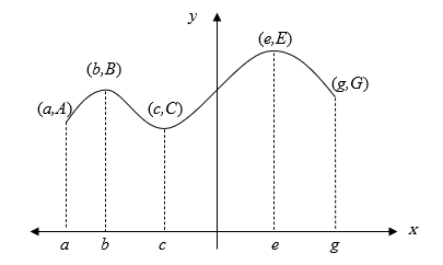
Figure 1. Sketch showing local and absolute minimums and maximums for a function.
Look at Figure 1, where if the domain D is given by the interval\(\ \left\lbrack a,g \right\rbrack,\) then C= absolute minimum of the function, as it is the smallest value of the function in the domain D. To find the absolute minimum of a continuous function with domain D, we look at the value of the function at the endpoints of D and also check where \(f^{\prime}(x) = 0\).
These points where\(f^{\prime}(x) = 0\) are critical points and could be local extreme (local minimum or local maximum) values. If \({ f}^{\prime\prime}\left( x \right) > 0\) at any of these points where local extremes occur, then it corresponds to a local minimum. Out of all the local minimums and the values at the domain ends, one can find the minimum of all such values. The point where this minimum exists is then the location of the absolute minimum value, and the value of the function at that point is the absolute minimum of the function.
Example 1
Find the location of the minimum of a polynomial \(25 - 20x + 4x^{2}.\)
Solution
\[\begin{split} f^{\prime}(x) &= \frac{d}{{dx}}(25 - 20x + 4x^{2})\\ &= \frac{d}{{dx}}(25) + \frac{d}{{dx}}( - 20x) + \frac{d}{{dx}}(4x^{2})\\ &= 0 - 20 + 4\frac{d}{{dx}}(x^{2})\\ &= - 20x + 4(2x)\\ &= - 20 + 8x \end{split}\]
Check where \(f^{\prime}(x) = 0\)
\[- 20 + 8x = 0\]
gives
\[\begin{split} x &= \frac{20}{8}\\ &= 2.5 \end{split}\]
Now check for \(f^{\prime\prime}(x)\)
\[\begin{split} f^{\prime}(x) &= - 20 + 8x\\ f^{\prime\prime}(x) &= \frac{d}{{dx}}( - 20 + 8x)\\ &= 8\\ f^{\prime\prime}(2.5) &= 8 \end{split}\]
Since \(f^{\prime}(2.5) = 0\) and\(f^{\prime\prime}(2.5) > 0\), the function has a local minimum at \(x = 2.5\). Is this point also the location of the absolute minimum? Yes, because of two reasons – firstly, the value of the function approaches infinity (maximum value) at the endpoints of the domain \(( - \infty,\infty)\). This check is made to look for extremes at the endpoints of the domain. Secondly, there is only one critical point at which \(f^{\prime}(x) = 0\) and \(f^{\prime\prime}(x) > 0\).
Example 2
Given \((x,y)\) data points \((5,10),\ (6,15),\ (10,20)\), and
\[S = \sum_{i = 1}^{3}{(y_{i} - ax_{i})^{2}}\] Find the value of \(a\) where the minimum of the summation series occurs.
Solution
The \((x,y)\) data pairs are given as follows
\[x_{1} = 5,\ x_{2} = 6,\ x_{3} = 10,\ y_{1} = 10,\ y_{2} = 15,\ y_{3} = 20\]
Calculating \(S\)
\[\begin{split} S &= \sum_{i = 1}^{3}{(y_{i} - ax_{i})^{2}}\\ &= (y_{1} - ax_{1})^{2} + (y_{2} - ax_{2})^{2} + (y_{3} - ax_{3})^{2}\\ &= (10 - 5a)^{2} + (15 - 6a)^{2} + (20 - 10a)^{2}\\ &= 161a^{2} - 680a + 725 \end{split}\]
Finding the first derivative
\[\begin{split} \frac{{dS}}{{da}} &= \frac{d}{{da}}(161a^{2} - 680a + 725)\\ &= 161(2a) - 680\\ &= 322a - 680 \end{split}\]
Using
\[\frac{{dS}}{{da}} = 0\]
gives
\[322a - 680 = 0\]
\[\begin{split} a &= \frac{680}{322}\\ &= 2.111 \end{split}\]
For the second derivative test
\[\begin{split} \frac{d^{2}S}{da^{2}} &= \frac{d}{{da}}\left( \frac{{dS}}{{da}} \right)\\ &= \frac{d}{{da}}(322a - 680)\\ &= 322 \end{split}\]
\[\frac{d^{2}S}{da^{2}}(2.11) = 322\]
Since,
\[\frac{{dS}}{{da}} = 0\ \text{at}\ a = 2.11\ \text{and}\]
\[\frac{d^{2}S}{da^{2}}(2.11) > 0.\]
a local minimum exists at \(a = 2.11\). Also, since \(S\) is a continuous function of \(a\) and it has only one point where \(\displaystyle \frac{{dS}}{{da}} = 0\) and \(\displaystyle \frac{d^{2}S}{da^{2}} > 0\), this local minimum is the absolute minimum.
Alternative Solution
Look at the solution if we had not expanded the summation.
\[S = \sum_{i = 1}^{n}{(y_{i} - ax_{i}})^{2}\]
Using the chain rule, if \(u\) is a function of variable \(a\)
\[\frac{d}{{da}}(u^{2}) = 2u\frac{{du}}{{da}}\]
then for
\[\frac{{dS}}{{da}} = 0\]
we get
\[\sum_{i = 1}^{n}{2(y_{i} - ax_{i}})( - x_{i}) = 0\]
\[\sum_{i = 1}^{n}{- 2y_{i}x_{i} + 2a{x_{i}}^{2}} = 0\]
\[\sum_{i = 1}^{3}{- 2y_{i}x_{i}} + \sum_{i = 1}^{3}{2a{x_{i}}^{2}} = 0\]
\[- 2\sum_{i = 1}^{3}{y_{i}x_{i}} + 2a\sum_{i = 1}^{3}{x_{i}}^{2} = 0\]
\[2a\sum_{i = 1}^{3}{x_{i}}^{2} = 2\sum_{i = 1}^{3}{y_{i}x_{i}}\]
\[a = \frac{\displaystyle\sum_{i = 1}^{3}{y_{i}x_{i}}}{\displaystyle \sum_{i = 1}^{3}{x_{i}}^{2}}\]
Substituting given values of \((x_i,y_i)\) gives
\[\begin{split} a &= \frac{(10 \times 5) + (15 \times 6) + (20 \times 10)}{5^{2} + 6^{2} + 10^{2}}\\ &= \frac{340}{161}\\ &= 2.11 \end{split}\]
We found
\[\frac{{dS}}{{da}} = \sum_{i = 1}^{3}{( - 2y_{i}x_{i}} + 2a{x_{i}}^{2})\]
Then
\[\begin{split} \frac{d^{2}S}{da^{2}} &= \sum_{i = 1}^{3}{2{x_{i}}^{2}}\\ &= 2(5)^{2} + 2(6)^{2} + 2(10)^{2}\\ &= 322 \end{split}\]
A local minimum hence exists at \(a = 2.11\). Also, since \(S\) is a continuous function of \(a\) and it has only one point where \(\displaystyle \frac{{dS}}{{da}} = 0\) and \(\displaystyle \frac{d^{2}S}{da^{2}} > 0\), this local minimum is the absolute minimum.
Learning Objectives
After successful completion of this lesson, you should be able to:
1) know the definition of a partial derivative,
2) find partial derivatives of a function.
Introduction
In regression, we are asked to find partial derivatives of functions. In this lesson, we cover the definition of a partial derivative and find partial derivatives of a simple function.
If someone gives a function \(f(x)\) of one variable \(x\), then we already know how to find the derivative \(f^{\prime}(x)\). However, functions can be of more than one independent variable. How can we then calculate the rate of change of a function with respect to each variable? This is simply done by defining partial derivatives, where one can find the derivative with respect to one variable while treating other variables as constants. For example, for a function \(f(x,y)\), the partial derivative with respect to \(x\) is defined as
\[\displaystyle \frac{\partial f}{\partial x} = \lim_{{\Delta x} \rightarrow 0}\frac{f(x + {\Delta x},y) - f(x,y)}{{\Delta x}}\;\;\;\;\;\;\;\;\;\;\;\; (1)\]
and the partial derivative with respect to \(y\) is defined as
\[\frac{\partial f}{\partial y} = \lim_{{\Delta y} \rightarrow 0}\frac{f(x,y + {\Delta y}) - f(x,y)}{{\Delta y}}\;\;\;\;\;\;\;\;\;\;\;\; (2)\]
Example 1
Given
\[f(x,y) = 2x^{3}y^{2} + 7x^{2}y^{2},\]
find
\[\frac{\partial f}{\partial x}\ \text{and}\ \frac{\partial f}{\partial y}.\]
Solution
\[f(x,y) = 2x^{3}y^{2} + 7x^{2}y^{2}\]
\[\frac{\partial f}{\partial x} = \frac{\partial}{\partial x}(2x^{3}y^{2} + 7x^{2}y^{2})\]
Since all variables other than \(x\) are considered to be constant,
\[\begin{split} \frac{\partial f}{\partial x} &= 2y^{2}\frac{\partial}{\partial x}(x^{3}) + 7y^{2}\frac{\partial}{\partial x}(x^{2})\\ &= 2y^{2}(3x^{2}) + 7y^{2}(2x)\\ &= 6x^{2}y^{2} + 14xy^{2} \end{split}\]
Now
\[\frac{\partial f}{\partial y} = \frac{\partial}{\partial y}(2x^{3}y^{2} + 7x^{2}y^{2})\]
Since all the variables other than \(y\) are considered to be constant,
\[\begin{split} \frac{\partial f}{\partial y} &= 2x^{3}\frac{\partial}{\partial y}(y^{2}) + 7x^{2}\frac{\partial}{\partial y}(y^{2})\\ &= 2x^{3}(2y) + 7x^{2}(2y)\\ &= 4x^{3}y + 14x^{2}y \end{split}\]
Learning Objectives
After successful completion of this lesson, you should be able to:
1) explain the first-order optimality condition,
2) apply the first-order optimality condition to find potential local minimums of a multivariant, continuous, and twice-differentiable function.
Recap: Local Minimum of a Single-Variant Function
In a previous lesson, we learned about the optimality conditions for finding extreme points and how to apply them to find a local minimum of a single-variant function. The optimality conditions are:
- First-order optimality condition: \(f^\prime\left( x \right) = 0\) (zero slope)
- Second-order optimality condition: \(f^{\prime\prime}\left( x \right) > 0\) (bowl-shaped, also called concave up)
Local Minimum of a Multivariant Function
The ideas for finding a local minimum of a multivariant function \(y = f(x_{1},x_{2},x_{3},\ldots,\ x_{n})\) are very similar to those for a single-variant function. The first-and second-order derivatives of the function can help us find local minimums.
First-Order Optimality Condition
The condition remains the same: \(f^{\prime}\left( x \right) = 0\), where \(x\) is a vector of \(n\) independent variables \((x_{1},x_{2},x_{3},\ldots,\ x_{n})\). However, since \(f(x)\) is now a multivariant function \(f\left( x \right) = f(x_{1},x_{2},x_{3},\ldots,\ x_{n})\), \(f^\prime(x)\) is now a vector, called gradient. Each element of the gradient vector is the corresponding partial derivative. The first-order optimality condition can now be more explicitly written as:
\[f^{\prime}\left( x \right) = \begin{pmatrix} \begin{matrix} \frac{\partial f}{\partial x_{1}} \\ \frac{\partial f}{\partial x_{2}} \\ \end{matrix} \\ \begin{matrix} \vdots \\ \frac{\partial f}{\partial x_{n}} \\ \end{matrix} \\ \end{pmatrix} = \begin{pmatrix} \begin{matrix} 0 \\ 0 \\ \end{matrix} \\ \begin{matrix} \vdots \\ 0 \\ \end{matrix} \\ \end{pmatrix}\;\;\;\;\;\;\;\;\;\;\;\; (1)\]
In other words, we have
\[\frac{\partial f}{\partial x_{i}} = 0,\ \forall i = 1,\ 2,\ldots,n\;\;\;\;\;\;\;\;\;\;\;\; (2)\]
where the symbol \(\forall\) means “for all.”
Second-Order Optimality Condition:
Similarly, the second-order optimality condition has to do with the second-order derivative of the function \(f^{\prime\prime}(x)\). For a multivariant function, its second-order derivative is defined by the Hessian matrix:
\[H\left( x \right) = \begin{bmatrix} \begin{matrix} \frac{\partial^{2}f}{\partial x_{1}^{2}} & \frac{\partial^{2}f}{\partial x_{1}\partial x_{2}} \\ \frac{\partial^{2}f}{\partial x_{2}\partial x_{1}} & \frac{\partial^{2}f}{\partial x_{2}^{2}} \\ \end{matrix} & \begin{matrix} \ \ \ \ \cdots & \frac{\partial^{2}f}{\partial x_{1}\partial x_{n}} \\ \ \ \ \ \cdots & \frac{\partial^{2}f}{\partial x_{2}\partial x_{n}} \\ \end{matrix} \\ \begin{matrix} \vdots & \vdots \\ \frac{\partial^{2}f}{\partial x_{n}\partial x_{1}} & \frac{\partial^{2}f}{\partial x_{n}\partial x_{2}} \\ \end{matrix} & \begin{matrix} \vdots & \vdots \\ \cdots & \frac{\partial^{2}f}{\partial x_{n}^{2}} \\ \end{matrix} \\ \end{bmatrix}\;\;\;\;\;\;\;\;\;\;\;\; (3)\]
The shape of the function is determined by the definiteness of \(H(x)\). The second-order optimality discussion is beyond the scope of this course.
.png)
Figure 1. The function f\(\left( x,y \right)\) has two global minima and one global maximum over its domain (Source: University Calculus by Hahn et al. Permission via Creative Commons License).
Critical Points of a Function of Two Variables
Let \(z = f(x,y)\) be a function of two variables \(x\) and \(y\). Then \(({x_{0}, y}_{0})\) is considered to be a critical point of \(f\) if \(f\) is differentiable on an open set that contains \(({x_{0},y}_{0})\) and if one of two conditions is true.
\[\begin{split} &(1)\ \ \left. \ \frac{\partial f}{\partial x} \right|_{{x_{0},y}_{0}} = 0;\ \left. \ \frac{\partial f}{\partial y} \right|_{{x_{0},y}_{0}} = 0\\ &(2)\ \ \left. \ \frac{\partial f}{\partial x} \right|_{x_{0},y_{0}}\text{or}\ \left. \ \frac{\partial f}{\partial y} \right|_{{x_{0},y}_{0}} \text{does not exist}\end{split}\;\;\;\;\;\;\;\;\;\;\;\; (4)\]
Example 1
Find the critical points of the function
\[f\left( x,y \right) = y^{4} + 8{xy} - 4y - 4x\]
Solution
Now
\[\begin{split} \frac{\partial f}{\partial x} &= \frac{\partial}{\partial x}\left( y^{4} + 8{xy} - 4y - 4x \right)\\ &= 8y - 4\\ \frac{\partial f}{\partial y} &= \frac{\partial}{\partial y}\left( y^{4} + 8{xy} - 4y - 4x \right)\\ &= {4y}^{3} + 8x - 4 \end{split}\]
Putting
\[\frac{\partial f}{\partial x} = 0\]
gives
\[8y - 4 = 0\]
\[\begin{split} y &= \frac{4}{8}\\ &= 0.5 \end{split}\]
Putting
\[\frac{\partial f}{\partial y} = 0\]
gives
\[{4y}^{3} + 8x - 4 = 0\]
\[x = \frac{4\ -\ 4y^{3}}{8}\]
Then at
\[y = 0.5\]
since
\[\frac{\partial f}{\partial y} = 0\]
we get
\[\begin{split} x &= \frac{4\ -\ 4{(0.5)}^{3}}{8}\\ &= 0.4375 \end{split}\]
Hence \((x,y) = (0.4375,\ 0.5)\) is a critical point of the function. This critical point could be corresponding to a local minimum, a local maximum, or a saddle point.
The following appendix is not used for the course but is included here for completion. It is the second derivative test that would establish if a critical point correspondence to a local minimum. And following that, one can find the absolute minimum by looking at all the local minima and the values of the function at the endpoints.
Appendix
Let \(z= f\left( x,y \right)\) be a function of two variables \(x\) and \(y\). Let the first and second-order partial derivatives be continuous on a domain containing (\({x_{0},y}_{0}\)). Then \(f(x,y)\) has a local minimum at \(({x_{0},y}_{0})\) if all the conditions below are met.
\[\left. \ \frac{\partial f}{\partial x} \right|_{{x_{0},y}_{0}} = 0,\ \text{and}\ \displaystyle \left. \ \frac{\partial f}{\partial y} \right|_{{x_{0},y}_{0}}\ \ = 0 ,\]
\[\left( \left. \ \frac{\partial^{2}f}{\partial x^{2}} \right|_{{x_{0},y}_{0}} \right)\left( \left. \ \frac{\partial^{2}f}{\partial y^{2}} \right|_{{x_{0},y}_{0}} \right) - \left( \left. \ \frac{\partial^{2}f}{\partial x\partial y} \right|_{{x_{0},y}_{0}} \right)^{2} > 0,\ \text{and}\]
\[\left. \ \frac{\partial^{2}f}{\partial x^{2}} \right|_{{x_{0},y}_{0}} > 0\;\;\;\;\;\;\;\;\;\;\;\; (A.1)\]
To find the absolute minimum, one needs to choose the smallest value amongst all the local minimums, and check the value of the function at the boundary of the domain.
Multiple Choice Test
(1). The average of 7 numbers is given \(12.6.\) If 6 of the numbers are \(5,\ 7,\ 9,\ 12,\ 17,\) and \(10\), the remaining number is
(A) \(-47.9\)
(B) \(-47.4\)
(C) \(15.6\)
(D) \(28.2\)
(2). The average and standard deviation of \(7\) numbers are given a \(8.142\) and \(5.005,\) respectively. If \(5\) numbers are \(5,\ 7,\ 9,\ 12,\) and \(17\), the other two numbers are
(A) \(- 0.1738,\ 7.175\)
(B) \(3.396,\ 12.890\)
(C) \(3.500,\ 3.500\)
(D) \(4.488,\ 2.512\)
(3). A local minimum of a continuous function in the interval (\(-\infty ,\infty\)) exists at \(x=a\) if
(A) \(f^{\prime}(a)=0, f^{\prime\prime}(a)=0\)
(B) \(f^{\prime}(a)=0, f^{\prime\prime}(a)<0\)
(C) \(f^{\prime}(a)=0, f^{\prime\prime}(a)>0\)
(D) \(f^{\prime}(a)=0, f^{\prime\prime}(a)\) does not exist
(4). The absolute minimum of a function \(f(x)=x^2+2x-15\) in the interval (\(-\infty, \infty\)) exists at \(x=\)________ and is ________.
(A) \(x=-1,f(-1)=-16\)
(B) \(x=-1,f(-1)=0\)
(C) \(x=3,f(3)=0\)
(D) \(x=5,f(5)=0\)
(5). The first order partial derivative with respect to \(x\) of \(u(x,y)=x^2y^3+6x^3e^{2y}\)
(A) \(y^3+6e^{2y}\)
(B) \(3x^2y^2+18x^3e^{2y}\)
(C) \(2xy^3+18x^2e^{2y}\)
(D) \(2xy^3+24x^2e^{2y}\)
(6). The critical point(s) \((x,y)\) of the function \(f(x,y)=y^3+4xy-16y-4x^2\) is (are)
(A) \((-4/3,1), (-8/3,2)\)
(B) \((4/3,8/3)\text{ and }(-1,-2)\)
(C) \((-4/3,-8/3)\text{ and }(1,2)\)
(D) \((0,0)\)
For the complete solution, go to
http://nm.mathforcollege.com/mcquizzes/06reg/quiz_06reg_background_solution_new.pdf
Problem Set
(1). Enumerate three items that a scientist should do for effective use of regression analysis.
(2). Enumerate three uses of regression analysis.
(3). Enumerate three common abuses of regression analysis.
(4). Does regression analysis prove causality? If not, what does it do.
(5). Give an example of each of abuses of regression – extrapolation, generalization, and misidentification.
(6). What are the differences between regression and interpolation?