Chapter 07.00: Physical Problem for Integration
Summary
The upward velocity of a rocket is given. To find the distance covered by the rocket requires integration.
Modeling
A rocket is going vertically up and expels fuel at a velocity \(2000\ \text{m/s}\) at a consumption rate of \(2100\ \text{kg/s}\). The initial mass of the rocket is \(140,000\ \text{kg}\). If the rocket starts from rest at \(t = 0\) seconds, how can I calculate the vertical distance covered by the rocket from \(t = 8\) to \(t = 30\) seconds?
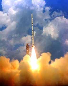
Figure 1 A rocket launched into space
If
\[m_{0} = \text{initial mass of rocket at}\ t = 0\ \text{(kg)}\]
\[q = \text{rate at which fuel is expelled (kg/sec)}\]
\[u = \text{velocity at which the fuel is being expelled (m/s)}\]
Then since fuel is expelled from the rocket, the mass of the rocket keeps decreasing with time. The mass of the rocket, \(m\) at any time \(t\)
\[m = m_{0} - {qt}\;\;\;\;\;\;\;\;\;\;\;\; (1)\]
The forces on the rocket at any time are found by applying Newton’s second law of motion. Then
\[\sum_{}^{}{F = ma}\;\;\;\;\;\;\;\;\;\;\;\; (2)\]
gives
\[{uq} - mg = ma\;\;\;\;\;\;\;\;\;\;\;\; (3)\]
Substituting Equation (1) in Equation (3) gives
\[{uq} - (m_{0} - qt)g = (m_{0} - qt)a\;\;\;\;\;\;\;\;\;\;\;\; (4)\]
where
\[g = \text{acceleration due to gravity (m/s}^{2})\]
Equation (4) is simplified to
\[a = \frac{{uq}}{m_{0} - {qt}} - g\;\;\;\;\;\;\;\;\;\;\;\; (5)\]
\[\frac{d^{2}x}{dt^{2}} = \frac{{uq}}{m_{0} - {qt}} - g\;\;\;\;\;\;\;\;\;\;\;\; (6)\]
\[\frac{{dx}}{{dt}} = - u\ln(m_{0} - qt) - gt + C\;\;\;\;\;\;\;\;\;\;\;\; (7)\]
Since the rocket starts from rest
\[\frac{{dx}}{{dt}} = 0\ \text{at}\ t = 0\]
\[0 = u\ln(m_{0}) + C\]
\[C = u\ln(m_{0})\]
Hence
\[\begin{split} \frac{{dx}}{{dt}} &= - u\ln(m_{0} - qt) - gt + u\ln(m_{0})\\ &= u\ln\left( \frac{m_{0}}{m_{0} - {qt}} \right) - {gt}\;\;\;\;\;\;\;\;\;\;\;\; (8) \end{split}\]
Then the distance covered by the rocket from \(t = t_{0}\) to \(t = t_{1}\) is,
\[x = \int_{t_{0}}^{t_{1}}{\left\lbrack u\ln\left( \frac{m_{0}}{m_{0} - {qt}} \right) - {gt} \right\rbrack{dt}}\;\;\;\;\;\;\;\;\;\;\;\; (9)\]
Let us substitute the values into the above equation. A rocket is going vertically up and expels fuel at a velocity \(2000\ \text{m/s}\) at a consumption rate of \(2100\ \text{kg/s}\). The initial mass of the rocket is \(140,000\ \text{kg}\). If the rocket starts from rest at \(t = 0\) seconds, how can I calculate the vertical distance covered by the rocket from \(t = 8\) to \(t = 30\) seconds?
Substituting
\[u = 2000\ \text{m/s}\]
\[m_{0} = 140000\ \text{kg}\]
\[q = 2100\ \text{kg/s}\]
\[g = 9.8\ \text{m/s}^2\]
\[t_{0} = 8\ \text{s}\]
\[t_{1} = 30\ \text{s}\]
\[x = \int_{8}^{30}{\left( 2000\ln\left\lbrack \frac{140000}{140000 - 2100t} \right\rbrack - 9.8t \right){dt}}\]
Modeling
Although a fuel cell provides DC electricity like an ordinary battery, it differs from an ordinary battery from the fact that its fuel source is externally supplied and as long as the fuel is being supplied, the fuel cell can in theory run continuously without needing a recharge. The two electrochemical reactions in a fuel cell occur at the electrodes (or poles) to which reactants are continuously fed. The reaction at the negative electrode (anode) is maintained by supplying a fuel such as hydrogen or methanol, whereas the positive electrode (cathode) reaction is maintained by the supply of oxygen or air. The two electrodes (anode and cathode) are separated by a proton conducting membrane – polymer electrolyte membrane (PEM).
A schematic diagram showing the operating principles of fuel cell that utilizes methanol as fuel, i.e., a Direct Methanol Fuel Cell (DMFC) is shown below.
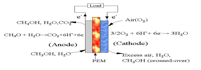
Figure 1. Direct methanol fuel cell
DC current is produced in the DMFC when methanol is electrochemically oxidized at the anode electrocatalyst. The electrons produced from the oxidation reaction leave the anode and travel through the external circuit to the cathode electrocatalyst where they are consumed together with oxygen in a reduction reaction. The circuit is maintained within the cell by the conduction of protons in the electrolyte (PEM).
Because of ease of design and its ability to withstand high temperature and pressure operation, most fuel cells today use PEM such as Nafion™.
The overall reaction occurring in the DMFC is equivalent to the direct combustion of methanol:
\[2CH_{3}OH + 3O_{2} \rightarrow 4H_{2}O + 2CO_{2}\]
One of the problems affecting the performance and hence commercialization of the direct methanol fuel cell (DMFC) is the depolarization of the oxygen reduction electrode caused by methanol cross-over. Depolarization as used here means that the presence of methanol limits the oxygen reduction and hence the amount of electricity produced. The exact role of methanol in limiting oxygen reduction can be inferred by understanding the physics and chemistry of the reaction. In an attempt to understand the mechanism of the depolarization process, an electro-kinetic model for mixed oxygen-methanol current on platinum was developed in our laboratory. A very simplified model [1] of the reaction developed suggests a functional relation of the form
\[T = - \int_{x_{1}}^{x_{2}}{\left( \frac{6.73x + 6.725 \times 10^{- 8} + 7.26 \times 10^{- 4}C_{{me}}}{3.62 \times 10^{- 12}x + 3.908 \times 10^{- 8}xC_{{me}}} \right){dx}}\]
where
\[T = \text{time},\ s\]
\[x = \text{Concentration of oxygen},\ {moles/c}{m}^{3},\]
\[C_{{me}} = \text{Concentration of methanol,}\ {moles/c}{m}^{3},\]
The parameters [1] in the above equation are
\[C_{{me}} = 5 \times 10^{- 4}{\ moles/c}{m}^{3}\]
The initial concentration is
\[x(t = 0) = 1.22 \times 10^{- 6}{\ moles/c}{m}^{3}\]
Questions
(1) Evaluate the time required for 50% of the initial oxygen concentration to be consumed in the fuel cell in the presence of methanol.
(2) Repeat (a) in the absence of methanol (that is, \(C_{{me}} = 0\)). What can you infer from the result in (a) and (b)?
(3) Plot time vs. oxygen concentration for the following concentrations of oxygen - \({x } = \ \lbrack{1.22, 1.20, 1.0, 0.8, 0.6, 0.4, 0.2}\rbrack \times {1}{0}^{{-6}}{moles/c}{m}^{3}\) both in the presence and absence of methanol.
References
[1] Itoe, R.N., Analysis of simultaneous oxygen reduction and methanol oxidation process in a direct methanol fuel cell, MS Thesis, Department of Chemical and Biomedical Engineering, Florida A&M University (1999).
Summary
Find if the concentration of benzene is above or below the toxicity limit at a critical distance from its source.
Modeling
In a class X528 well in New York State, you are asked to find if the concentration of benzene is below the toxicity level of \(0.5{mg/l}\) at a distance of \(36m\) from the point of contamination. The contamination at the source is constant at \(3.5{mg/l}\) for a whole year.
The equations governing transport of groundwater contaminant are quite complex. They depend on several parameters such as “the molecular diffusion of the contaminant, physical and chemical isotropy of the medium, and actual direction of the groundwater flow” [1].
Here we consider that the groundwater is flowing in one-direction, \(x\) and the aquifer has isotropic and homogeneous physical and chemical characteristics. In that case, the governing equation [2] for the concentration \(c\left( x,t \right)\) of the contaminant is given by
\[\frac{\partial c}{\partial t} + u\frac{\partial c}{\partial x} = D\frac{\partial^{2}c}{\partial x^{2}}\ \ \ (1)\]
where
\[u = \text{velocity of ground water flow in the}\ x\ \text{-direction}\ ({m/s})\]
\[t = \text{time}\ (s)\]
\[x = \text{distance from source}\ (m)\]
\[D = \text{dispersion coefficient}\ \left( m^{2} \right).\]
To solve this partial differential equation (1) [3], we use Laplace transforms. Applying Laplace transform to both sides on the variable \(t\),
\[L\left( \frac{\partial c}{\partial t} + u\frac{\partial c}{\partial x} \right) = L\left( D\frac{\partial^{2}c}{\partial x^{2}} \right)\]
\[sC - c\left( x,0 \right) + u\frac{{dC}}{{dx}} = D\frac{d^{2}C}{dx^{2}}\ \ \ (2)\]
where
\[L\lbrack c(x,t)\rbrack = C\left( x,s \right)\]
Since the initial concentration is zero,
\[c\left( x,0 \right) = 0,\]
Equation (2) becomes
\[sC + u\frac{{dc}}{{dx}} = D\frac{d^{2}C}{dx^{2}}\]
\[D\frac{d^{2}C}{dx^{2}} - u\frac{{dC}}{{dx}} - sC = 0\ \ \ (3)\]
This is a homogenous ordinary differential equation. It is linear with fixed coefficients. The characteristics equation of the above ordinary differential equation (3) is
\[Dm^{2} - {um} - s = 0\]
\[m = \frac{u \pm \sqrt{u^{2} + 4Ds}}{2D}\ \ \ (4)\]
The homogeneous as well as the complete solution of Equation (3) is
\[C\left( x,s \right) = A\left( s \right)e^{\frac{u + \sqrt{u^{2} + 4Ds}}{2D}x} + B\left( s \right)e^{\frac{u - \sqrt{u^{2} + 4Ds}}{2D}x}\ \ \ (5)\]
At \(x = \infty\), that is far away from the source, the concentration of the pollutant is zero, that is \(c\left( \infty,s \right) = 0\), that is, \(C\left( \infty,s \right) = 0\). This forces \(A\left( s \right) = 0\)as the exponent of the exponential term is always positive as \(u,D,s > 0\). The exponent of the exponential term on the second term will be negative as \(\sqrt{u^{2} + uDs} > u\)for all values of \(u,D,s\)as \(u,D,s > 0\). Equation (5) hence reduces to
\[C\left( x,s \right) = B\left( s \right)e^{\frac{u - \sqrt{u^{2} + 4Ds}}{2D}x}\ \ \ (6)\]
At \(x = 0\), \(c = c_{0}\) (initial concentration, \(c_{0}\)), then \(C\left( 0,s \right) = \frac{c_{0}}{s}\). Substituting this in equation (6) gives
\[\frac{c_{o}}{s} = B\left( s \right)\]
then equation (6) is
\[\begin{split} C\left( x,s \right) &= \frac{c_{0}}{s}e^{\frac{u - \sqrt{u^{2} + 4Ds}}{2D}x}\\ &= \left( c_{0}e^{\frac{{ux}}{2D}} \right)\left( \frac{e^{- \frac{\sqrt{u^{2} + 4Ds}}{2D}x}}{s} \right) \end{split}\]
\[L^{- 1}\lbrack C(x,s)\rbrack = L^{- 1}\left\lbrack \left( c_{0}e^{\frac{{ux}}{2D}} \right)\left( \frac{e^{- \frac{\sqrt{u^{2} + 4Ds}}{2D}x}}{s} \right) \right\rbrack\]
\[\begin{split} c\left( x,t \right) &= c_{0}e^{\frac{{ux}}{2D}}L^{- 1}\left( \frac{e^{- \frac{\sqrt{u^{2} + 4Ds}}{2D}x}}{s} \right)\\ &= C_{0}e^{\frac{{ux}}{2D}}L^{- 1}\left\lbrack \frac{e^{- \frac{x}{\sqrt{D}}\sqrt{\frac{u^{2}}{4D} + s}}}{S} \right\rbrack\ \ \ (7) \end{split}\]
Let
\[a = \frac{x}{\sqrt{D}}\]
\[b = \frac{u}{2\sqrt{D}}\]
Then Equation (7) becomes
\[c\left( x,t \right) = c_{0}e^{{ab}}L^{- 1}\left( \frac{e^{- a\sqrt{b^{2} + s}}}{s} \right)\ \ \ (8)\]
Using the formulas
\[L^{- 1}(e^{- a\sqrt{s}}) = \left( \frac{a}{2\sqrt{\pi t^{3}}}e^{- \frac{a^{2}}{4t}} \right),a > 0,\] and
\[L^{- 1}\left( F\left( s + a \right) \right) = e^{- {at}}f\left( t \right)\]
then
\[L^{- 1}\left( e^{- a\sqrt{b^{2} + s}} \right) = \frac{a}{2\sqrt{\pi t^{3}}}e^{- \frac{a^{2}}{4t} - b^{2}t}\ \ \ (9)\]
Then from
\[\int_{0}^{t}f\left( \tau \right)d\tau = \frac{F\left( s \right)}{s}\]
we get
\[\begin{split} L^{- 1}\left( \frac{e^{- a\sqrt{b^{2} + s}}}{s} \right) &= \int_{0}^{t}\frac{a}{2\sqrt{\pi\tau^{3}}}e^{- \frac{a^{2}}{4\tau}}e^{- b^{2}\tau}{d\tau}\\ &= e^{- {ab}}\int_{0}^{t}\frac{a}{2\sqrt{\pi\tau^{3}}}e^{- \frac{\left( a - 2b\tau \right)^{2}}{4\tau}}{d\tau}\\ &= e^{- {ab}}\int_{0}^{t}\left( \frac{a + 2b\tau}{4\sqrt{\pi\tau^{3}}} + \frac{a - 2b\tau}{4\sqrt{\pi\tau^{3}}} \right)e^{- \frac{\left( a - 2b\tau \right)^{2}}{4\tau}}{d\tau}\\ &= e^{- {ab}}\int_{0}^{t}\frac{a + 2b\tau}{4\sqrt{\pi\tau^{3}}}e^{- \frac{\left( a - 2b\tau \right)^{2}}{4\tau}}d\tau + e^{- {ab}}\int_{0}^{t}{\frac{a - 2b\tau}{4\sqrt{\pi\tau^{3}}}e^{- \frac{\left( a - 2b\tau \right)^{2}}{4\tau}}}\\ &= e^{- {ab}}\int_{0}^{t}\frac{a + 2b\tau}{4\sqrt{\pi\tau^{3}}}e^{- \frac{\left( a - 2b\tau \right)^{2}}{4\tau}}d\tau + e^{- {ab}}\int_{0}^{t}{\frac{a - 2b\tau}{4\sqrt{\pi\tau^{3}}}e^{- \frac{\left( a - 2b\tau \right)^{2}}{4\tau} - \frac{8ab\tau}{4\tau} + \frac{8ab\tau}{4\tau}}}\\ &= e^{- {ab}}\int_{0}^{t}\frac{a + 2b\tau}{4\sqrt{\pi\tau^{3}}}e^{- \frac{\left( a - 2b\tau \right)^{2}}{4\tau}}d\tau + e^{{ab}}\int_{0}^{t}{\frac{a - 2b\tau}{4\sqrt{\pi\tau^{3}}}e^{- \frac{\left( a + 2b\tau \right)^{2}}{4\tau}}{d\tau}} \end{split}\]
Let
\[p = \frac{a - 2b\tau}{\sqrt{4\tau}},\]
\[q = \frac{a + 2b\tau}{\sqrt{4\tau}}\]
then
\[\begin{split} L^{- 1}\left( \frac{e^{- a\sqrt{b^{2} + s}}}{s} \right) &= \frac{e^{- {ab}}}{\sqrt{\pi}}\int_{\infty}^{\frac{a - 2bt}{\sqrt{4t}}}{e^{- p^{2}}{dp} - \frac{e^{{ab}}}{\sqrt{\pi}}\int_{\infty}^{\frac{a + 2bt}{\sqrt{4t}}}{e^{- q^{2}}{dq}}}\\ &= \frac{e^{- {ab}}}{2}{erfc}\left( \frac{a - 2bt}{2\sqrt{t}} \right) + \frac{e^{{ab}}}{2}{erfc}\left( \frac{a + 2bt}{2\sqrt{t}} \right)\ \ \ (10) \end{split}\]
Using Equation (10), Equation (8) becomes
\[\begin{split}c\left( x,t \right) &= c_{0}e^{{ab}}\left\lbrack \frac{e^{- {ab}}}{2}{erfc}\left( \frac{a - 2bt}{2\sqrt{t}} \right) + \frac{e^{{ab}}}{2}{erfc}\left( \frac{a + 2bt}{2\sqrt{t}} \right) \right\rbrack\\ &= \frac{c_{0}}{2}\left\lbrack {erfc}\left( \frac{a - 2bt}{2\sqrt{t}} \right) + \frac{e^{2ab}}{2}{erfc}\left( \frac{a + 2bt}{2\sqrt{t}} \right) \right\rbrack\ \ \ (11) \end{split}\]
Substituting back
\[a = - \frac{x}{\sqrt{D}},\]
\[b = \frac{u}{2\sqrt{D}}\]
\[c\left( x,t \right) = \frac{c_{0}}{2}\left\lbrack {erfc}\left( \frac{x - {ut}}{2\sqrt{{Dt}}} \right) + e^{\frac{{ux}}{D}}{erfc}\left( \frac{x + ut}{2\sqrt{{Dt}}} \right) \right\rbrack\ \ \ (12)\]
The velocity of the ground flow, \(u\) is given by
\[u = \frac{k}{n_{{ed}}}\frac{dh}{dl}\ \ \ (13)\]
where
\[n_{{ed}}= \text{effective Darcian porosity,}\]
\[K = \text{permeability,}\]
\[\frac{dh}{{dl}} =\text{ground water gradient.}\]
Assuming
\[n_{{ed}}= 22\% = 0.22\]
\[K = 0.002 \frac{{cm}}{s}\]
\[\frac{dh}{{dl}} = 0.01\frac{{cm}}{{cm}}.\]
Then from Equation (13),
\[\begin{split} u &= \frac{0.002}{0.22}(0.01)\\ &= 9.091 \times 10^{- 5}\frac{{cm}}{s}. \end{split}\]
So in the formula for concentration given by Equation (12), substituting
\[D = 0.01\frac{{c}{m}^{2}}{s}\]
\[c_{0} = 3.5\frac{{mg}}{L}\]
\[x = 36m\]
\[t = 1\text{ year} = 3.15 \times 10^{7}s\]
the concentration of benzene after 1 year at a distance of \(36m\)is
\[\begin{split} c &= \frac{3.5}{2}{erfc}\left( \frac{36 - \left( 9.091 \times 10^{- 5} \right)\left( 3.15 \times 10^{7} \right)}{2\sqrt{\left( 0.01 \right)\left( 3.15 \times 10^{7} \right)}} \right)+\\& \ \ \ \ \ \frac{3.5}{2} e^{\frac{\left( 9.091\times 10^{- 5} \right)\left( 36 \right)}{0.01}}{erfc}\left( \frac{36 + \left( 9.091 \times 10^{- 5} \right)\left( 3.15 \times 10^{7} \right)}{2\sqrt{\left( 0.01 \right)\left( 3.15 \times 10^{7} \right)}} \right) \\ &= 1.75\lbrack erfc\left( 0.6560 \right) + e^{32.73}{erfc}\left( 5.758 \right)\rbrack\ \ \ (14) \end{split}\]
As you can see to calculate the concentration of benzene at \(x = 36m\), we need to calculate \({erfc}\left( 0.6560 \right)\) and \({erfc}\left( 5.758 \right)\). How is \({erfc}\left( x \right)\) defined?
\[{erfc}\left( x \right) = \int_{\infty}^{x}e^{- z^{2}}{dz}\]
So
\[{erfc}\left( 0.6560 \right) = \int_{\infty}^{0.6560}e^{- z^{2}}{dz}\]
Since \(e^{- z^{2}}\)decays rapidly as \(z \rightarrow \infty\), we will approximate
\[{erfc}\left( 0.6560 \right) = \int_{5}^{0.6560}{e^{- z^{2}}{dz}}\]
So to find whether the concentration of benzene is below toxicity level, we need to find the integral numerically.
Questions
(1) What is the concentration of benzene after 2 years?
(2) After 1 year, at what distance does the concentration go below the toxicity level of 0.5 mg/L?
References
(1) EPA Region 5 Water Draft UIC Class IV and V Site Assessment Guidelines, http://www.epa.gov/R5water/uic/r5guid/siteasst.htm, last accessed July 2004.
(2) Fetter, C.W., Jr., Applied Hydrology, Merill Publishing Co, Columbus, 1980.
(3) Li, W., Differential Equations of Hydraulic Transients, Dispersion, and Groundwater Flow, Prentice Hall, Englewood Cliffs, NJ, 1972
Modeling
Human vision has the remarkable ability to infer 3D shapes from 2D images. When we look at 2D photographs or TV we do not see them as 2D shapes, rather as 3D entities with surfaces and volumes. Perception research has unraveled many of the cues that are used by us. The intriguing question is: can we replicate some of these abilities on a computer? To this end, in this assignment we are going to look at one way to engineer a solution to the 3D shape from 2D images problem. Apart from the pure fun of solving a new problem, there are many practical applications of this technology such as in automated inspection of machine parts, inference of obstructing surfaces for robot navigation, and even in robot-assisted surgery.
Image is a collection of gray level values at a set of predetermined sites known as pixels, arranged in an array. These gray level values are also known as image intensities. The registered intensity at an image pixel is dependent on a number of factors such as the lighting conditions, surface orientation, and surface material properties. The nature of lighting and its placement can drastically affect the appearance of a scene. In another module on simultaneous linear equations, we saw how to infer the surface normal vectors for each point in the scene, given three images of the scene taken with three different light sources. In Figure 1 we see vector field that we have inferred form the three images. In this module, we will see how we can integrate this vector field to arrive at a surface.
To be able to reconstruct the shape of the underlying surface, we have to first understand the how the surface normal is related to the underlying surface. Figure 2 shows the schematic of the camera centered coordinate axis that we can use to formulate the problem. The \(z\) -direction is away from the camera towards the scene. Let the scene surface be parameterized by the function.
\[z = g(x,y)\]
The equation of the local surface normal can be related to this function as follows. If we find two tangents on the surface then the cross product of these tangents will give us the surface normal. Two tangents along the \(x\) and \(y\) -directions can easily be specified in terms of the derivatives along these directions. Figure 2 shows the underlying geometry that can be used to arrive at these equations.
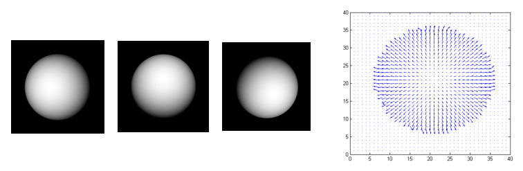
Figure 1. The first three images are of a sphere taken with three different light source positions. The right image is a vector field representation of the surface normal vectors estimated from these three images. Can you compute the underlying surface representation from this vector field?
\[{\overrightarrow{t}}_{x} = \begin{bmatrix} 1 \\ 0 \\ \frac{\partial g(x,y)}{\partial x} \\ \end{bmatrix}\ \text{and}\ {\overrightarrow{t}}_{y} = \begin{bmatrix} 0 \\ 1 \\ \frac{\partial g(x,y)}{\partial y} \\ \end{bmatrix} \]
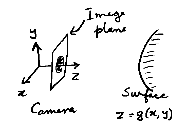
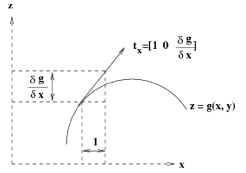
Figure 2. Relationship between surface tangent at a point to underlying surface equation. On the top is a simplified representation of the imaging geometry. The surface is assumed to be far away from the camera. On the bottom is a schematic of the local geometry on the scene surface.
The local surface normal, \(n\), will be along the direction of the cross product of \(t_{x}\) and \(t_{y}\).
\[c\overrightarrow{n} = - {\overrightarrow{t}}_{x} \times {\overrightarrow{t}}_{y} = \begin{bmatrix} \frac{\partial g(x,y)}{\partial x} \\ \frac{\partial g(x,y)}{\partial x} \\ - 1 \\ \end{bmatrix}\]
Note that there is \(1800\) ambiguity in the specification of the surface normal. We need the negative sign because we want the surface normal to be oriented towards the camera and the \(z\) -axis is pointed away from the camera. Also, note that the cross product gives as a vector along the surface normal. We have to normalize the vector to arrive at the surface normal. For notational ease let
\[p = \frac{\partial g(x,y)}{\partial x} \ \text{and}\] \[q = \frac{\partial g(x,y)}{\partial y}\]
Then,
\[\overrightarrow{n} = \begin{bmatrix} n_{x} \\ n_{y} \\ n_{z} \\ \end{bmatrix} = \frac{1}{\sqrt{p^{2} + q^{2} + 1}}\begin{bmatrix} p \\ q \\ - 1 \\ \end{bmatrix}\]
We see that the surface normal can be expressed in terms of the derivatives of the underlying surface. From this equation, we can express the local surface derivatives in terms of ratios of the surface normal components.
\[\frac{\partial g(x,y)}{\partial x} = \frac{n_{x}}{n_{y}}\ \text{and}\] \[\frac{\partial g(x,y)}{\partial y} = \frac{n_{y}}{n_{z}}\]
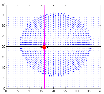
Figure 3. Integration paths to arrive at the depth surface value for the point marked by the red dot.
The black lines denote possible paths over which the x-partial derivative can be integrated. And, the purple lines denote possible paths to integrate the y-partial derivative. The paths are shown overlaid on the input vector field representing the partial derivatives of the surface along x and y directions.
We arrive at the final surface equation by integration these partial derivatives. Since we have a 2D field, we can perform the integration along many paths. The simplest paths are along the \(x\) (or \(y\)) axis.
\[g(u,v) = \int_{o}^{u}{\frac{\partial g(x,v)}{\partial x}{dx}}\ \text{or}\]
\[g(u,v) = \int_{o}^{v}{\frac{\partial g(u,y)}{\partial y}{dy}}\]
One could also start from the right edge of the image and integrate the partial derivative with respect to \(x\) towards the left edge, or start from the bottom of the image and integrate the \(y\) -partial derivative towards the top. These directions are depicted in Figure 3. The equivalent integrals are as follows. The image is assumed to N pixels by M pixels in size and the negative sign arises because of the direction of the integration.
\[g(u,v) = - \int_{N}^{u}{\frac{\partial g(x,v)}{\partial x}{dx}}\ \text{or}\]
\[g(u,v) = - \int_{M}^{v}{\frac{\partial g(u,y)}{\partial y}{dy}}\]
Ideally, all the four integrals should result in the same value, however, for noisy, real world data they will never be the same. One solution is to take the average of these four integrals as the final value. Note that these integrals have to be evaluated for each location \((u,v)\) in the image to arrive at the full surface.
Worked Out Example
Consider the problem of estimating the surface height along the line passing through the center of the sphere in Figure 1. Figure 4 (a) shows the input estimates for the partial derivatives along the x direction, \(\displaystyle p = \frac{\partial g(x,y)}{\partial x}\) for the sphere along this line. The raw data for this plot is given below.
| x | g |
|---|---|
| \(1.00000\) | \(0.00000\) |
| \(2.00000\) | \(0.00000\) |
| \(3.00000\) | \(0.00000\) |
| \(4.00000\) | \(0.00000\) |
| \(5.00000\) | \(0.00000\) |
| \(6.00000\) | \(0.00000\) |
| \(7.00000\) | \(0.00000\) |
| \(8.00000\) | \(0.00000\) |
| \(9.00000\) | \(0.00000\) |
| \(10.00000\) | \(0.00000\) |
| \(11.00000\) | \(0.00000\) |
| \(12.00000\) | \(0.00000\) |
| \(13.00000\) | \(0.00000\) |
| \(14.00000\) | \(0.00000\) |
| \(15.00000\) | \(0.00000\) |
| \(16.00000\) | \(0.00000\) |
| \(17.00000\) | \(0.00000\) |
| \(18.00000\) | \(0.00000\) |
| \(19.00000\) | \(0.00000\) |
| \(20.00000\) | \(0.00000\) |
| \(21.00000\) | \(0.00000\) |
| \(22.00000\) | \(0.00000\) |
| \(23.00000\) | \(0.00000\) |
| \(24.00000\) | \(0.00000\) |
| \(25.00000\) | \(0.00000\) |
| \(26.00000\) | \(0.00000\) |
| \(27.00000\) | \(0.00000\) |
| \(28.00000\) | \(0.00000\) |
| \(29.00000\) | \(0.00000\) |
| \(30.00000\) | \(5.42857\) |
| \(31.00000\) | \(4.40000\) |
| \(32.00000\) | \(3.82362\) |
| \(33.00000\) | \(3.23097\) |
| \(34.00000\) | \(2.74844\) |
| \(35.00000\) | \(2.43579\) |
| \(36.00000\) | \(2.19293\) |
| \(37.00000\) | \(2.04677\) |
| \(38.00000\) | \(1.91851\) |
| \(39.00000\) | \(1.88649\) |
| \(40.00000\) | \(1.62019\) |
| \(41.00000\) | \(1.55007\) |
| \(42.00000\) | \(1.47428\) |
| \(43.00000\) | \(1.44755\) |
| \(44.00000\) | \(1.36134\) |
| \(45.00000\) | \(1.28187\) |
| \(46.00000\) | \(1.14868\) |
| \(47.00000\) | \(1.15089\) |
| \(48.00000\) | \(1.14027\) |
| \(49.00000\) | \(1.05379\) |
| \(50.00000\) | \(0.98459\) |
| \(51.00000\) | \(1.00329\) |
| \(52.00000\) | \(0.96249\) |
| \(53.00000\) | \(0.90161\) |
| \(54.00000\) | \(0.88597\) |
| \(55.00000\) | \(0.83243\) |
| \(56.00000\) | \(0.78901\) |
| \(57.00000\) | \(0.80149\) |
| \(58.00000\) | \(0.74730\) |
| \(59.00000\) | \(0.73934\) |
| \(60.00000\) | \(0.70364\) |
| \(61.00000\) | \(0.67288\) |
| \(62.00000\) | \(0.66161\) |
| \(63.00000\) | \(0.62773\) |
| \(64.00000\) | \(0.61402\) |
| \(65.00000\) | \(0.60783\) |
| \(66.00000\) | \(0.58271\) |
| \(67.00000\) | \(0.55106\) |
| \(68.00000\) | \(0.52999\) |
| \(69.00000\) | \(0.50641\) |
| \(70.00000\) | \(0.50146\) |
| \(71.00000\) | \(0.46053\) |
| \(72.00000\) | \(0.45829\) |
| \(73.00000\) | \(0.43148\) |
| \(74.00000\) | \(0.41627\) |
| \(75.00000\) | \(0.39025\) |
| \(76.00000\) | \(0.38186\) |
| \(77.00000\) | \(0.35635\) |
| \(78.00000\) | \(0.34187\) |
| \(79.00000\) | \(0.32304\) |
| \(80.00000\) | \(0.31064\) |
| \(81.00000\) | \(0.27967\) |
| \(82.00000\) | \(0.27367\) |
| \(83.00000\) | \(0.26137\) |
| \(84.00000\) | \(0.24340\) |
| \(85.00000\) | \(0.23128\) |
| \(86.00000\) | \(0.20758\) |
| \(87.00000\) | \(0.19566\) |
| \(88.00000\) | \(0.19566\) |
| \(89.00000\) | \(0.17807\) |
| \(90.00000\) | \(0.16632\) |
| \(91.00000\) | \(0.14409\) |
| \(92.00000\) | \(0.12686\) |
| \(93.00000\) | \(0.11039\) |
| \(94.00000\) | \(0.10481\) |
| \(95.00000\) | \(0.08266\) |
| \(96.00000\) | \(0.06623\) |
| \(97.00000\) | \(0.04945\) |
| \(98.00000\) | \(0.04383\) |
| \(99.00000\) | \(0.03309\) |
| \(100.00000\) | \(0.00038\) |
| \(101.00000\) | \(-0.00516\) |
| \(102.00000\) | \(-0.02149\) |
| \(103.00000\) | \(-0.03232\) |
| \(104.00000\) | \(-0.04317\) |
| \(105.00000\) | \(-0.05421\) |
| \(106.00000\) | \(-0.06513\) |
| \(107.00000\) | \(-0.09250\) |
| \(108.00000\) | \(-0.09820\) |
| \(109.00000\) | \(-0.11468\) |
| \(110.00000\) | \(-0.12011\) |
| \(111.00000\) | \(-0.13697\) |
| \(112.00000\) | \(-0.14808\) |
| \(113.00000\) | \(-0.18176\) |
| \(114.00000\) | \(-0.18776\) |
| \(115.00000\) | \(-0.19904\) |
| \(116.00000\) | \(-0.20511\) |
| \(117.00000\) | \(-0.22784\) |
| \(118.00000\) | \(-0.25084\) |
| \(119.00000\) | \(-0.26862\) |
| \(120.00000\) | \(-0.26960\) |
| \(121.00000\) | \(-0.30463\) |
| \(122.00000\) | \(-0.30577\) |
| \(123.00000\) | \(-0.33591\) |
| \(124.00000\) | \(-0.33720\) |
| \(125.00000\) | \(-0.35061\) |
| \(126.00000\) | \(-0.37626\) |
| \(127.00000\) | \(-0.38823\) |
| \(128.00000\) | \(-0.40213\) |
| \(129.00000\) | \(-0.42330\) |
| \(130.00000\) | \(-0.44994\) |
| \(131.00000\) | \(-0.47173\) |
| \(132.00000\) | \(-0.47897\) |
| \(133.00000\) | \(-0.50129\) |
| \(134.00000\) | \(-0.54231\) |
| \(135.00000\) | \(-0.54480\) |
| \(136.00000\) | \(-0.57621\) |
| \(137.00000\) | \(-0.56790\) |
| \(138.00000\) | \(-0.61925\) |
| \(139.00000\) | \(-0.63884\) |
| \(140.00000\) | \(-0.65569\) |
| \(141.00000\) | \(-0.68145\) |
| \(142.00000\) | \(-0.73088\) |
| \(143.00000\) | \(-0.75263\) |
| \(144.00000\) | \(-0.76928\) |
| \(145.00000\) | \(-0.79030\) |
| \(146.00000\) | \(-0.80970\) |
| \(147.00000\) | \(-0.81065\) |
| \(148.00000\) | \(-0.88367\) |
| \(149.00000\) | \(-0.89782\) |
| \(150.00000\) | \(-0.92400\) |
| \(151.00000\) | \(-1.00067\) |
| \(152.00000\) | \(-1.03536\) |
| \(153.00000\) | \(-1.08947\) |
| \(154.00000\) | \(-1.09584\) |
| \(155.00000\) | \(-1.20465\) |
| \(156.00000\) | \(-1.22123\) |
| \(157.00000\) | \(-1.26090\) |
| \(158.00000\) | \(-1.30056\) |
| \(159.00000\) | \(-1.33557\) |
| \(160.00000\) | \(-1.49718\) |
| \(161.00000\) | \(-1.53483\) |
| \(162.00000\) | \(-1.70123\) |
| \(163.00000\) | \(-1.69167\) |
| \(164.00000\) | \(-1.89507\) |
| \(165.00000\) | \(-2.06525\) |
| \(166.00000\) | \(-2.24788\) |
| \(167.00000\) | \(-2.45874\) |
| \(168.00000\) | \(-2.80478\) |
| \(169.00000\) | \(-3.22446\) |
| \(170.00000\) | \(-3.86839\) |
| \(171.00000\) | \(-4.00000\) |
| \(172.00000\) | \(-4.00000\) |
| \(173.00000\) | \(0.00000\) |
| \(174.00000\) | \(0.00000\) |
| \(175.00000\) | \(0.00000\) |
| \(176.00000\) | \(0.00000\) |
| \(177.00000\) | \(0.00000\) |
| \(178.00000\) | \(0.00000\) |
| \(179.00000\) | \(0.00000\) |
| \(180.00000\) | \(0.00000\) |
| \(181.00000\) | \(0.00000\) |
| \(182.00000\) | \(0.00000\) |
| \(183.00000\) | \(0.00000\) |
| \(184.00000\) | \(0.00000\) |
| \(185.00000\) | \(0.00000\) |
| \(186.00000\) | \(0.00000\) |
| \(187.00000\) | \(0.00000\) |
| \(188.00000\) | \(0.00000\) |
| \(189.00000\) | \(0.00000\) |
| \(190.00000\) | \(0.00000\) |
| \(191.00000\) | \(0.00000\) |
| \(192.00000\) | \(0.00000\) |
| \(193.00000\) | \(0.00000\) |
| \(194.00000\) | \(0.00000\) |
| \(195.00000\) | \(0.00000\) |
| \(196.00000\) | \(0.00000\) |
| \(197.00000\) | \(0.00000\) |
| \(198.00000\) | \(0.00000\) |
| \(199.00000\) | \(0.00000\) |
| \(200.00000\) | \(0.00000\) |
This data needs to be numerically integrated to arrive at height values. Figure 4 (b) shows the plot of the surface height, as computed by integrating starting from left and from right. We used the trapezoidal integration method. Notice the small discrepancy, which is due to real world data noise. The overall shape does look circular, which should serve as a sanity check on the calculations.
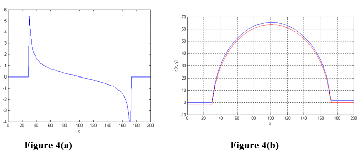
Figure 4. (a) The plot of the estimates for the partial derivatives along the x direction, \(p = \frac{\partial g(x,y)}{\partial x}\) for the sphere along a horizontal line passing through the middle of the sphere. (b) Plot of the integrated value at each point along the horizontal. The blue plot corresponds to integrating from left to right and the red plot corresponds to integrating from right to left.
If we repeat the above process along the vertical direction (along image columns), then we will arrive at two more estimates for the middle point of the sphere, which can be averaged to arrive at one estimate. If we repeat this for each point on the sphere, not just the middle, then we will arrive at the surface representation for the full sphere. Figure 5 shows the averaged estimate of the sphere as estimated from the input vector field. Note the spherical nature of the final estimate.
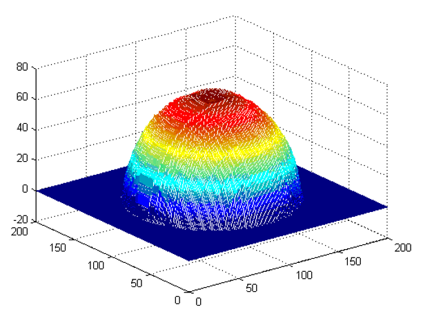
Figure 5. Estimated surface height for the vector field in Figure 1(c) as computed by averaging the estimates of the integrals along four directions, for each point.
Questions
(1) Write code to recover the surface height at each point in the image given the vector field.
(2) For any point on the sphere, specify 25 different paths along which you can integrate.
(3) Study how the roughness of the estimated surface changes with number of path integrals that are averaged.
Summary
Not all electrical components, especially off-the-shelf components match their nominal value. Variations in materials and manufacturing as well as operating conditions can affect their value. Suppose a circuit is designed such that it requires a specific component value, how confident can we be that the variation in the component value will result in acceptable circuit behavior? To solve this problem a probability density function will need to be integrated to determine the confidence interval.
Modeling
Today’s consumer products rely heavily on small electronic circuits to provide much of their functionality. Each of these circuits is built around electrical components that, like all devices, vary in value due to variations in materials, manufacturing, and operating conditions. For example, capacitors are notoriously variable often operating as much as \(+ / - 20\%\) from their nominal value. Clearly, a variation in capacitor value can have an affect on the operation of an electronic circuit. If the statistical properties of the capacitor and resistor value distributions are known, stochastic methods can be used to compute this effect. Unfortunately, this is often not the case and we are frequently left to use empirical methods to determine this effect. A common technique is to use a Monte Carlo method where a circuit will be built (or simulated) many times with different components from a lot and the resulting behavior analyzed. The goal will be to determine a confidence value that a randomly selected circuit built with these components will behave within a certain interval.
Consider the case of an op-amp based square wave generator as shown in Figure 1. Its operative behavior in terms of period is described by the equation [1, pp. 625-627]
\[T = 2RC\ln\left( 1 + 2\frac{R_{2}}{R_{1}} \right)\]
Clearly, the period/frequency of this circuit is quite susceptible to variations in all the components \(1\) except the op-amp, resistor, \(R_{3}\) and the zener diodes. How then can the likely behavior to all the possible combination of variations in the components \(R,C,R_{1}\) and \(R_{2}\) be determined? The answer is to apply a Monte Carlo method and some basic statistics.
If we assume that the statistical distribution of the circuit behavior is normal[1] then a two-tailed confidence interval test can be used to determine the likelihood that the circuit will behave acceptably [2, pp. 113-27]. An examination of the literature will show that a confidence interval can be established through the use of the z-test. For a sample of size n with known standard deviation \(\sigma\) it can be determined with confidence \(\left( 1 - \alpha \right)\) that the measured value will stay in the following range
\[\bar{x} - z\left( \alpha/2 \right)\sigma < value < \bar{x} + z\left( \alpha/2 \right)\sigma,\]
where
\[\overline{x}\ \text{is the sample mean of the measured value.}\]
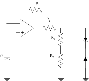
Figure 1 Square-Wave Oscillator
If \(\alpha\) is \(0.05\) then there is \(90\%\) confidence that the value of all possible circuits will be within the indicated range about the sample mean. When the sample size \(n\) is smaller than \(30\) or the population standard deviation,\(\sigma\) is not known the sample standard deviation,\(s\) can be substituted and the normal distribution must be replaced with the Student-T distribution [2, pp. 174-7].
Interpretation of the term \(z\left( \alpha/2 \right)\) and \(t\left( \alpha/2,n - 2 \right)\) often leads to a lot of confusion. It is the \(z -\) or \(t -\) score value that is necessary so that \(\left( 1 - \alpha \right)\) of the area under the probability distribution is inside the desired range. This is often referred to, in part, as a two-tailed test. Figure 2 shows this graphically.
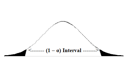
Figure 2 \(\left( 1 - \alpha \right)\) Confidence Interval
\(z\left( \alpha/2 \right)\) is the value so that when the normal distribution is integrated from \(- z\left( \alpha/2 \right)\ \text{to} + z\left( \alpha/2 \right)\) that the resulting area is\(\left( 1 - \alpha \right)\). This integration is summarized by the following equation.
\[\left( 1 - \alpha \right) = \int_{- z\left( \alpha/2 \right)}^{z\left( \alpha/2 \right)}{\frac{1}{\sqrt{2\pi}}e^{- \frac{x^{2}}{2}}{dx}}\]
The analysis is similar for the Student-T distribution and \(t\left( \alpha/2,n - 2 \right)\).
The problem is that there is no closed-form solution to the integration of either the normal distribution or the Student-T distribution. These are typically handled via look-up tables of the cumulative distributions from \(- \infty\) to \(z\) [2, pp. 513-14].
In the case of a confidence interval computation generally everything is known except for \(z\left( \alpha/2 \right)\). However, in the case of a circuit, that analysis can be reversed to determine with what confidence the average circuit behavior will be in a given interval. In other words, suppose that the goal is to determine how likely it is that the square-wave generator for Figure 1 will behave with a frequency of \(11\) kHz. For example, suppose that suitable components have been chosen for \(R,C,R_{1}\ \)and\(\ R_{2}\) for a lot and that \(25\)circuits were built with the following results being measured:
\[\text{Number of Samples:}\ n = 25\]
\[\text{Average Period:}\ \bar{x} = 0.995{ms}\]
\[\text{Standard Deviation:}\ \sigma = 0.02{ms}\]
What is the likelihood, with this batch of components, that any given oscillator will have its frequency within \(5\%\) of the target of \(1{kHz}\)? Rearranging the confidence interval formula and solving for \(z\left( \alpha/2 \right)\) yields the following two equations. One for the upper end for \(\mu < 1.053{ms}\) and the other for the upper end for\(\mu > 0.952{m}{s}^{3}\).
\[z\left( \alpha_{1}/2 \right) = \frac{\left( \mu_{1} - \bar{x} \right)}{\sigma} = \frac{\left( 1.053m - 0.995m \right)}{0.02m} = 2.9\]
\[z\left( \alpha_{2}/2 \right) = \frac{\left( \mu_{2} - \bar{x} \right)}{\sigma} = \frac{\left( 0.952m - 0.995m \right)}{0.02m} = - 2.15\]
The likelihood of this happening can then be determined by finding the total area under the normal distribution for the range in question
\[\left( 1 - \alpha \right) = \int_{- 2.15}^{2.9}{\frac{1}{\sqrt{2\pi}}e^{- \frac{x^{2}}{2}}{dx}}\]
Questions
(1) There is no real way to know the population standard deviation, \(\sigma\), so the more complex formula using the sample standard deviation, \(s\) , and the Student-T distribution would have to be used, especially when \(n\) is less than \(30\) 30 [2, pp. 174-19]. The entire analysis is the same except the integral is now the more complicated.
\[\left( 1 - \alpha \right) = \int_{- t\left( \alpha/2,m \right)}^{t\left( \alpha/2,m \right)}{\left\{ \frac{\Gamma\left( \frac{m + 1}{2} \right)}{\sqrt{{m\pi}}\Gamma\left( \frac{m}{2} \right)}\left( 1 + \frac{x^{2}}{m} \right)^{- \left( \frac{m + 1}{2} \right)} \right\}{dx}}\]
where
\[\Gamma\left( 1 \right) = 1\]
\[\Gamma\left( 1/2 \right) = \sqrt{\pi}\]
\[\Gamma\left( m \right) = \left( m - 1 \right)\Gamma\left( m - 1 \right)\]
Perform the computations using the Student-T distribution.
(2) The more common way of using these statistics is to compute the actual confidence interval centered about the sample data. This means that \(\alpha\) is known and \(z\left( \alpha/2 \right)\) or \(t\left( \alpha/2,n - 2 \right)\) have to be computed. This can be done by repeatedly trying possible values for \(z\) or \(t\) and evaluating the integral. This is an excellent application for a root-finding algorithm. If an algorithm like bisection method of solving nonlinear equations were used, how would you pick the initial bounds for the \(x\) or \(t\) value?
(3) Because there are actual formulas for the functional inside the integral and not just sampled points on the curve in question, it is possible to apply an interval halving approach and a Romberg extrapolation to solve these integrals. Set up the algorithm for doing this.
(4) Normal and Student-T distribution tables like those in [2, pp. 513-4] are limited in their choices. Integrating these distributions from \(- \infty\) can be used to generate a more complete table. To do this an algorithm must take advantage of the symmetry in the distributions since it is not possible to integrate numerically with an infinite bound. When the \(z\) or \(t\) value is less than zero simply report \(0.5\) minus the integral from 0 to \(z\)or \(t\), and when the \(z\)or \(t\) value is greater than zero simply report \(0.5\) plus the integral from \(0\) to \(z\) or \(t\). Set-up the algorithm for doing this.
(5) In the analysis above it was assumed that the population of circuits was roughly normal, this should generally be tested before applying the assumption. There exist goodness-of-fit tests to see if the population is sufficiently normal. For more information, see [2, pp. 265-8].
References
[1] Millman, J., Micro-Electronics: Digital and Analog Circuits and Systems, McGraw Hill, 1979.
[2] Walpole, R. and Myers, R., Probability and Statistics for Engineers and Scientists, 2nd Ed., MacMillan, 1978.
Summary
The number of sheets in a roll of toilet paper are sampled at a factory. Even if the number of the sheets in every chosen sample turns out to be what is advertised or more, the probability of every roll having the advertised number or more sheets is not \(100\%\). To find out this probability requires numerical integration.
Modeling
An industrial engineer works as a quality control engineer for a company making toilet paper. The company advertises that every roll of toilet paper has at least \(250\) sheets. It is the industrial (quality) engineer’s responsibility to validate this claim by sampling rolls off of the assembly line and determining the probability (that is, confidence) that the company can make a claim. Note that validating the claim is important to avoid frivolous lawsuits associated with false advertising.
Let us assume that the number of sheets in a roll of toilet paper, \(y\), is governed by the normal probability distribution (see figure on next page), that is,
\[y \sim N(\mu,\sigma^{2})\;\;\;\;\;\;\;\;\;\;\;\; (1)\]
where N is a normal random variable described by its mean, \(\mu\) , and standard deviation, \(\sigma\). The probability distribution function of the normal random variable \(y\) is
\[f(y) = \frac{1}{\sigma\sqrt{2\pi}}e^{-(1/2)\left\lbrack y - \mu)/\sigma \right\rbrack^{2}}\;\;\;\;\;\;\;\;\;\;\;\; (2)\]
and is shown in Figure 1.
Note that the previously described normal probability density function was first derived by Abraham de Moivre in 1733 in his book called The Doctrine of Chance. Initially, the discovery went unnoticed until it was re-derived by Laplace and Gauss about 50 years later. Hence, it is often called the Gaussian distribution. The normal probability distribution, which is a continuous distribution, is derived from the binomial probability distribution, which is a discrete distribution. The discrete binomial distribution is given below
\[f(y) =\frac{n!}{k!\left( n - k \right)!}p^{k}\left( 1 - p \right)^{n - k}\;\;\;\;\;\;\;\;\;\;\;\; (3)\]
where \(n\) is the number of samples and \(k\) is the number of successes with a probability of \(p\). When \(n\) is large, the binomial distribution approaches the normal distribution. In fact, when \(n\) is greater than or equal to \(6\), the normal distribution is an excellent approximation to the binomial distribution (Figure 2).
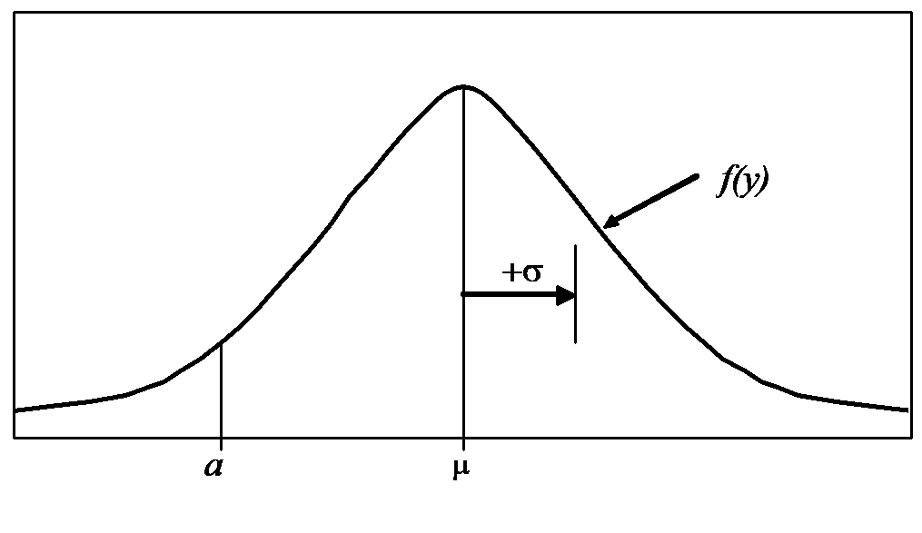
Figure 1 Probability distribution function,
\(\displaystyle f(y) = \frac{1}{\sigma\sqrt{2\pi}}e^{- (1/2)\left\lbrack y - \mu)/\sigma \right\rbrack^{2}}\)
The actual proof that the binomial distribution approaches the normal distribution involves a special case of the central limit theorem and is beyond the scope of this problem. Furthermore, the derivation also involves the inclusion of a continuity correction factor.
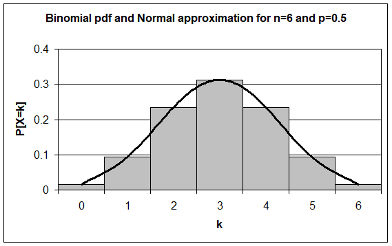
Figure 2 Binomial pdf and normal approximation for \(n = 6\) and \(p = 0.5\)
Since the quality engineer cannot sample every roll of toilet paper and count the number of sheets, the mean and standard deviation are estimated based on a sample size of \(n\) rolls of toilet paper. The mean, \(\bar{y}\), and standard deviation, \(s\), of the sample (that is, the sample mean and sample standard deviation) are estimates of the actual mean, \(\mu\), and standard deviation, \(\sigma\), and are given by
\[\bar{y} = \frac{\displaystyle \sum_{i = 1}^{n}y_{i}}{n} \approx \mu\;\;\;\;\;\;\;\;\;\;\;\; (4)\]
\[s = \sqrt{\frac{\displaystyle \sum_{i = 1}^{n}\left( y_{i} - \bar{y} \right)^{2}}{n - 1}} \approx \sigma\;\;\;\;\;\;\;\;\;\;\;\; (5)\]
where \(n\) is the number of samples (that is, rolls of toilet paper). The probability that the number of sheets in a roll is greater than or equal to some specified number, \(a\), is the area under the probability density function (that is, integral) from \(a\) to \(\infty\), and is given by
\[\begin{split} P(y \geq a) &= \int_{a}^{\infty}{f(y)dy}\\ &= \int_{a}^{\infty}{\frac{1}{\sigma\sqrt{2\pi}}e^{- (1/2)\left\lbrack (y - \mu)/\sigma \right\rbrack^{2}}{dy}}\;\;\;\;\;\;\;\;\;\;\;\; (6) \end{split}\]
Note that the result of Equation (6) is a number from \(0\) to \(1\) that correlates to a \(0\%\) to \(100\%\) probability, respectively.
A co-operative education student working for an industrial (quality) engineer samples \(10\) rolls of toilet paper every week and determines that the number of sheets in each roll is
| Roll | Number of sheets |
|---|---|
| \(1\) | \(253\) |
| \(2\) | \(250\) |
| \(3\) | \(251\) |
| \(4\) | \(252\) |
| \(5\) | \(253\) |
| \(6\) | \(253\) |
| \(7\) | \(252\) |
| \(8\) | \(254\) |
| \(9\) | \(252\) |
| \(10\) | \(252\) |
The industrial (quality) engineer calculates the following mean and standard deviation of the sample of 10 rolls of toilet paper.
\[\bar{y} = \frac{253 + 250 + 251 + 252 + 253 + 253 + 252 + 254 + 252 + 252}{10} = 252.2 \approx \mu\]
\[s = \sqrt{\frac{\begin{matrix} \ &\left( 253 - 252.2 \right)^{2} + \left( 250 - 252.2 \right)^{2} + \left( 251 - 252.2 \right)^{2} + \\ \ &\left( 252 - 252.2 \right)^{2} + \left( 253 - 252.2 \right)^{2} + \left( 253 - 252.2 \right)^{2} + \\ \ &\left( 252 - 252.2 \right)^{2} + \left( 254 - 252.2 \right)^{2} + \left( 252 - 252.2 \right)^{2} + \left( 252 - 252.2 \right)^{2} \\ \end{matrix}}{10 - 1}} = 1.135 \approx \sigma\]
Using Equation (6), the probability that the number of sheets in a roll is greater than or equal to \(250\) sheets is
\[P(y \geq 250) = \int_{250}^{\infty}{\frac{1}{1.135\sqrt{2\pi}}e^{- (1/2)\left\lbrack (y - 252.2)/1.135 \right\rbrack^{2}}{dy}}\]
\[P(y \geq 250) = \int_{250}^{\infty}{0.3515e^{- 0.3881(y - 252.2)^{2}}{dy}}\]
\[P(y \geq 250) = ??\]
Questions
(1) Although all the rolls have more than \(250\) sheets, why do we not get a \(100\%\) probability that all the rolls have \(250\) sheets or more?
(2) Change one of the data points to \(248\) sheets and rework the problem.
(3) To find the integral numerically in Equation (6), one may substitute infinity by \(5\). How will you justify this substitution quantitatively?
Summary
To find the diametrical contraction during shrink-fitting in a trunnion requires one to first find how the coefficient of linear thermal expansion of steel is related to temperature. The relation may be given through a second-order polynomial. This model is then used in integration to find the diametrical contraction.
Modeling
To make the fulcrum (Figure 1) of a bascule bridge, a long hollow steel shaft called the trunnion is shrink fit into a steel hub. The resulting steel trunnion-hub assembly is then shrink fit into the girder of the bridge.
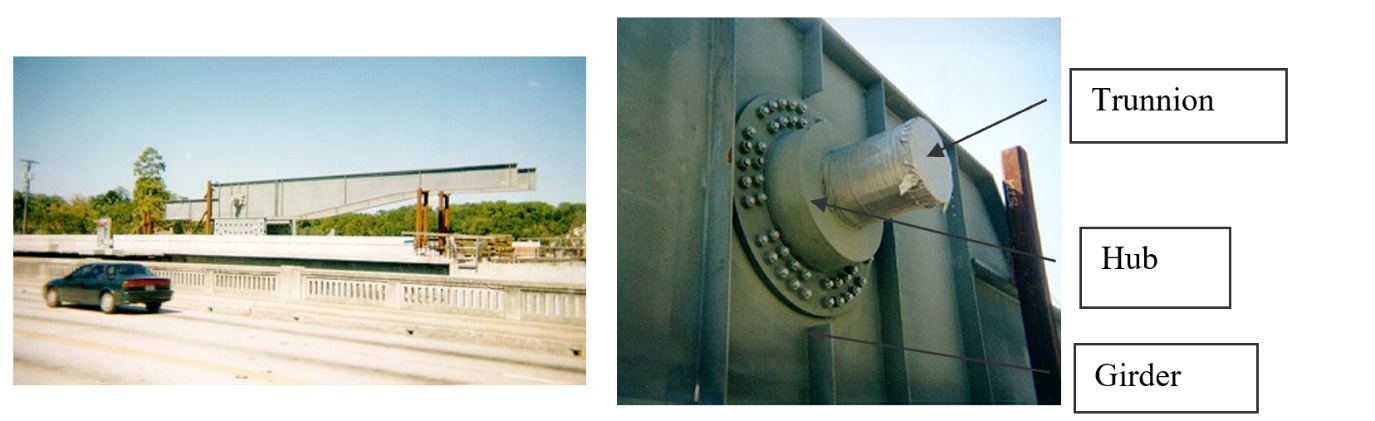
Figure 1 Trunnion-Hub-Girder (THG) assembly.
This is done by first immersing the trunnion in a cold medium such as a dry-ice/alcohol mixture. After the trunnion reaches the steady-state temperature, that is, the temperature of the cold medium, the trunnion outer diameter contracts. The trunnion is taken out of the medium and slid though the hole of the hub (Figure 2).
When the trunnion heats up, it expands and creates an interference fit with the hub. In 1995, on one of the bridges in Florida, this assembly procedure did not work as designed. Before the trunnion could be inserted fully into the hub, the trunnion got stuck. Luckily the trunnion was taken out before it got stuck permanently. Otherwise, a new trunnion and hub would be needed to be ordered at a cost of $50,000. Coupled with construction delays, the total loss could have been more than a hundred thousand dollars.
Why did the trunnion get stuck? This failure took place because the trunnion had not contracted enough to slide through the hole. Can you find out why?
A hollow trunnion of outside diameter \({12.36}{3}^{\prime\prime}\) is to be fitted in a hub of inner diameter \(12.358^{\prime\prime}\). The trunnion was put in a dry ice/alcohol mixture (temperature of the fluid - dry ice/alcohol mixture is \(- 108{^\circ}\text{F}\)) to contract the trunnion so that it can be slid through the hole of the hub. To slide the trunnion without sticking, a diametrical clearance of at least \(0.01^{\prime\prime}\) is required between the trunnion and the hub. Assuming the room temperature is \(80{^\circ}\text{F}\), is immersing it in a dry-ice/alcohol mixture a correct decision?
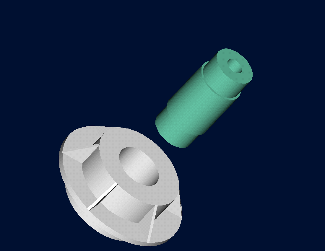
Figure 2 Trunnion slided through the hub after contracting
To calculate the contraction in the diameter of the trunnion, the coefficient of linear thermal expansion at room temperature is used. In that case, the reduction, \({\Delta D}\) in the outer diameter of the trunnion is
\[\Delta D = D\alpha\Delta T\;\;\;\;\;\;\;\;\;\;\;\; (1)\]
where
\[D = \text{outer diameter of the trunnion,}\]
\[\alpha =\text{coefficient of linear thermal expansion at room temperature, and}\]
\[\Delta T =\text{change in temperature,}\]
Given
\[D = 12.363^{\prime\prime}\]
\[\alpha = 6.817 \times 10^{- 6}\ \text{in/in/}{^\circ}\text{F}\ \text{at}\ 80{^\circ}\text{F}\]
\[\begin{split} \Delta T &=T_{{fluid}} - T_{{room}}\\ &= - 188{^\circ}\text{F} \end{split}\]
where
\[T_{{fluid}} = \text{temperature of dry-ice/alcohol mixture,}\]
\[T_{{room}}= \text{room temperature,}\]
the reduction in the trunnion outer diameter is given by
\[\begin{split} \Delta D &= (12.363)\left( 6.47 \times 10^{- 6} \right)\left( - 188 \right)\\ &= - 0.01504^{\prime\prime} \end{split}\]
So the trunnion is predicted to reduce in diameter by \(0.01504^{\prime\prime}\). But is this enough reduction in diameter? As per specifications, he needs the trunnion to contract by
\[\begin{split} &= \text{trunnion outside diameter} - \text{hub inner diameter} + \text{diametral clearance}\\ &= 12.363^{\prime\prime} - 12.358^{\prime\prime} + 0.01^{\prime\prime}\\ &= 0.015^{\prime\prime} \end{split}\]
So, according to his calculations, immersing the steel trunnion in a dry-ice/alcohol mixture gives the desired contraction of \(0.015^{\prime\prime}\) as we predict a contraction of \(0.01504^{\prime\prime}\).
But as shown in Figure 3, the coefficient of linear thermal expansion of steel decreases with temperature and is not constant over the range of temperature the trunnion goes through. Hence the above formula (Equation (1)) would overestimate the thermal contraction.
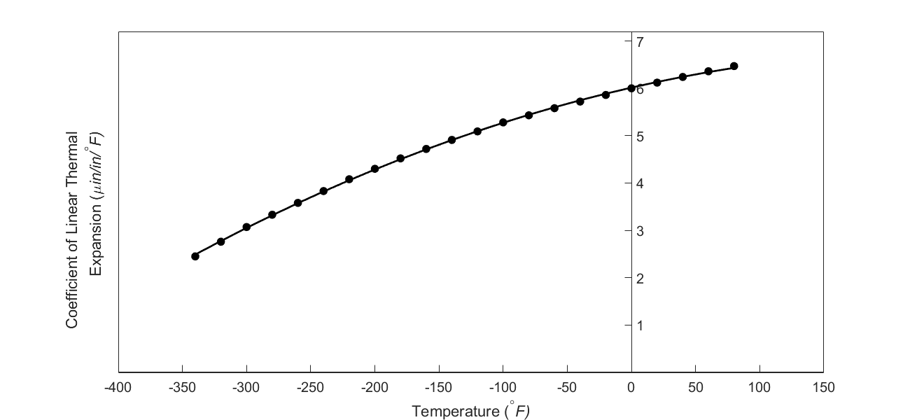 Figure 3 Varying coefficient of linear thermal expansion as a
function of temperature for cast steel.
Figure 3 Varying coefficient of linear thermal expansion as a
function of temperature for cast steel.
The contraction in the diameter for the trunnion for which the thermal expansion coefficient varies as a function of temperature is given by
\[\Delta D = D\int_{T_{{room}}}^{T_{{fluid}}}{\alpha dT}\;\;\;\;\;\;\;\;\;\;\;\; (2)\]
Note that Equation (2) reduces to Equation (1) if the coefficient of thermal expansion is assumed to be constant. In Figure 3, the coefficient of linear thermal expansion of typical cast steel is approximated by a second-order polynomial as
\[\alpha = - 1.2278 \times 10^{- 11}T^{2} + 6.1946 \times 10^{- 9}T + 6.0150 \times 10^{- 6}\;\;\;\;\;\;\;\;\;\;\;\; (3)\]
From Equations (2) and (3)
\[\Delta D = 12.363\int_{80}^{- 108}{\left( - 1.2278 \times 10^{- 11}T^{2} + 6.1946 \times 10^{- 9}T + 6.015 \times 10^{- 6} \right){dT}}\;\;\;\;\;\;\;\;\;\;\;\; (4)\]
Questions
(1) Can you now find the contraction of the trunnion outer diameter?
(2) Is the magnitude of contraction more than \(0.015^{\prime\prime}\) as required?
(3) If that is not the case, what if the trunnion were immersed in liquid nitrogen (boiling temperature=\(- 321{^\circ}\text{F}\))? Will that give enough contraction in the trunnion?
(4) Rather than regressing the data to a second-order polynomial so that one can find the contraction in the trunnion outer diameter, how would you use the trapezoidal rule of integration for unequal segments? What is the relative difference between the two results? The data for the coefficient of linear thermal expansion as a function of temperature is given below.
Table 1 coefficient of linear thermal expansion as a function of temperature.
| Temperature | Coefficient of Thermal Expansion |
|---|---|
| \({^\circ}\text{F}\) | \(\mu\text{in/in/}{^\circ}\text{F}\) |
| \(80\) | \(6.47\) |
| \(60\) | \(6.36\) |
| \(40\) | \(6.24\) |
| \(20\) | \(6.12\) |
| \(0\) | \(6.00\) |
| \(-20\) | \(5.86\) |
| \(-40\) | \(5.72\) |
| \(-60\) | \(5.58\) |
| \(-80\) | \(5.43\) |
| \(-100\) | \(5.28\) |
| \(-120\) | \(5.09\) |
| \(-140\) | \(4.91\) |
| \(-160\) | \(4.72\) |
| \(-180\) | \(4.52\) |
| \(-200\) | \(4.30\) |
| \(-220\) | \(4.08\) |
| \(-240\) | \(3.83\) |
| \(-260\) | \(3.58\) |
| \(-280\) | \(3.33\) |
| \(-300\) | \(3.07\) |
| \(-320\) | \(2.76\) |
| \(-340\) | \(2.45\) |
The second-order polynomial is derived using regression analysis which is another mathematical process where numerical methods are employed. Regression analysis approximates discrete data such as the coefficient of linear thermal expansion vs. temperature data as a continuous function. This is an excellent example of where one has to use numerical methods for more than one process to solve a real-life problem.