Chapter 05.05: Spline Method of Interpolation
Learning Objectives
After successful completion of this lesson, you should be able to:
1) justify why higher-order interpolation is a bad idea,
2) how spline interpolation can avoid the pitfalls of higher-order interpolation.
Introduction
Polynomial interpolation involves finding a polynomial of order \(n\) or less that passes through the \(n + 1\) points. Several methods to obtain such a polynomial include the direct method (also called the Vandermonde polynomial method), Newton’s divided difference polynomial method, and the Lagrangian interpolation method.
So is the spline method yet another method of obtaining this \(n^{\text{th}}\) order polynomial. …… NO!
Actually, when \(n\) becomes large, in many cases, one may get oscillatory behavior in the interpolating polynomial. This phenomenon was illustrated by Runge when he interpolated data based on a simple function of
\[y = \frac{1}{1 + 25x^{2}} \;\;\;\;\;\;\;\;\;\;\;\; (1)\]
on an interval of \([-1, 1]\).
For example, take six equidistantly spaced points in \([-1, 1]\) and find \(y\) at these points from Equation (1). These values are given in Table 1.
Table 1. Six equidistantly spaced points in \([-1, 1]\).
| \(x\) | \(\displaystyle y = \frac{1}{1 + 25x^{2}}\) |
|---|---|
| \(-1.0\) | \(0.038461\) |
| \(-0.6\) | \(0.1\) |
| \(-0.2\) | \(0.5\) |
| \(0.2\) | \(0.5\) |
| \(0.6\) | \(0.1\) |
| \(1.0\) | \(0.038461\) |
Now through these six data points, one can pass a fifth-order interpolating polynomial.
\[\begin{split} f_{5}(x) &= 1.2019x^{4}- 1.7308x^{2}+ 0.56731,\ - 1 \leq x \leq 1 \end{split} \;\;\;\;\;\;\;\;\;\;\;\;(2)\]
On plotting (Figure 1) the fifth-order polynomial (Equation (2)) and the original function (Equation (1)), you can see that they do not match well. The polynomial does go through the six data pairs of Table 1, but it does not even come close to the original function at many other points. Just look at \(x = 0.85\), the value of the original function is \(0.052459,\) but the fifth-order polynomial gives you a value of \(-0.055762\). That is a whopping relative true error of \(206.30\%\).
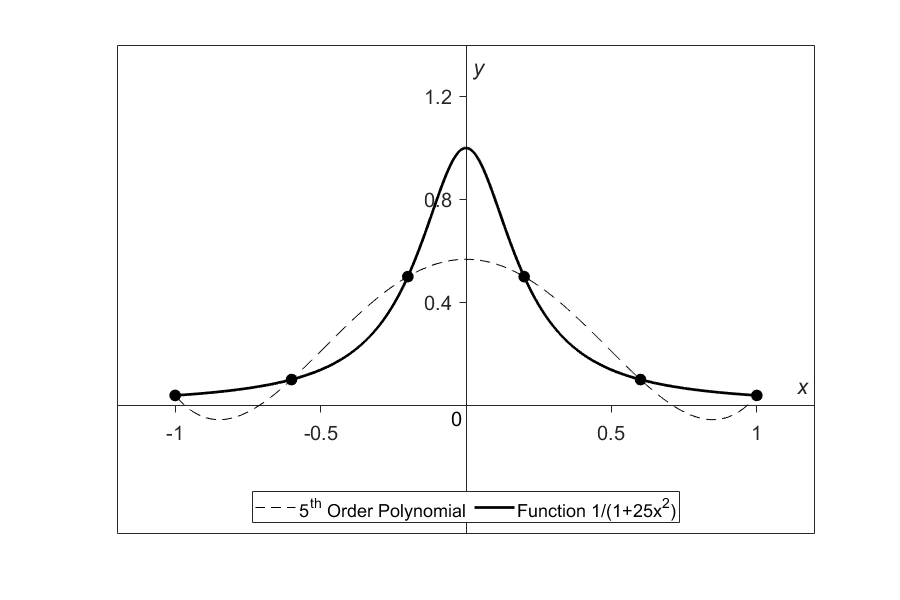
Figure 1. Fifth order polynomial interpolation with six equidistant points.
One may think that choosing more points in the interval \([-1, 1]\) will give us a better match between the original function and the interpolant, but it diverges even more (Figure 2). Here \(20\) equidistant points were chosen in the interval \([-1, 1]\) to draw a \(19^{th}\) order interpolating polynomial. It, however, did do a better job of approximating the data but except near the ends where the approximation is worse than before. At our chosen point, \(x = 0.85\), the value of the original function is \(0.052459\), while we get \(-0.62944\) from the \(19^{th}\) order polynomial. That gives a big whopper relative true error of \(1299.9\)%.
In fact, Runge found that as the order of the polynomial approaches infinity, the polynomial diverges even more in the interval of \(- 1 < x < - 0.726\) and \(0.726 < x < 1\).
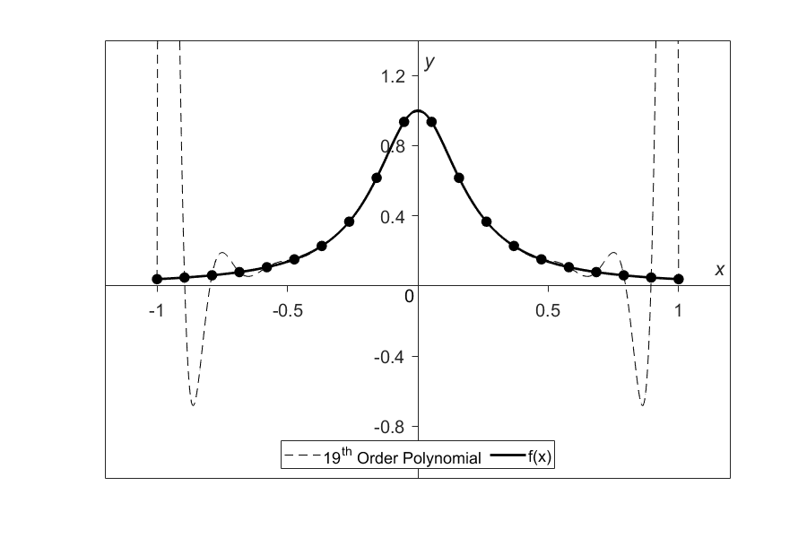
Figure 2. Nineteenth order polynomial interpolation with twenty equidistant points
So, what is the solution to using information from more data points, but at the same time keeping the function reasonably true to the data behavior? The answer is in spline interpolation and will be discussed in the following lessons. The most common types of spline interpolation used are linear, quadratic, and cubic.
Learning Objectives
After successful completion of this lesson, you should be able to:
1) develop linear spline interpolant to given data points,
2) estimate unknown data points from the linear spline interpolant.
Linear Spline Interpolation
Given \(\left( x_{0},y_{0} \right),\left( x_{1},y_{1} \right),\ldots\dots,\left( x_{n - 1},y_{n - 1} \right),\left( x_{n},y_{n} \right)\), find the interpolating linear spline (Figure 1) to the data. This procedure simply involves drawing straight lines between consecutive points.
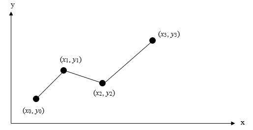
Figure 1. Linear splines.
Assuming that the above data is given in ascending order, the interpolating linear spline, also called spline of degree 1, \(f(x)\) is given by \[\begin{split} f(x) &= f(x_{0}) + \frac{f(x_{1}) - f(x_{0})}{x_{1} - x_{0}}(x - x_{0}),\ x_{0} \leq x \leq x_{1},\\ &= f(x_{1}) + \frac{f(x_{2}) - f(x_{1})}{x_{2} - x_{1}}(x - x_{1}),\ x_{1} \leq x \leq x_{2},\\ &\ \ \ \ \ \vdots\\ &= f(x_{n - 1}) + \frac{f(x_{n}) - f(x_{n - 1})}{x_{n} - x_{n - 1}}(x - x_{n - 1}),\ x_{n - 1} \leq x \leq x_{n}. \end{split}\;\;\;\;\;\;\;\;\;\;\;\; (1)\]
Note that \(y_i=f(x_i)\) in the above expression and that the terms of
\[\frac{f(x_{i}) - f(x_{i - 1})}{x_{i} - x_{i - 1}}\;\;\;\;\;\;\;\;\;\;\;\; (2)\]
are simply slopes between \(x_{i - 1}\) and \(x_{i}\).
Example 1
The upward velocity of a rocket is given as a function of time in Table 1 (Figure 2).
Table 1. Velocity as a function of time.
| \(t\ (\text{s})\) | \(v(t)\ (\text{m/s})\) |
|---|---|
| \(0\) | \(0\) |
| \(10\) | \(227.04\) |
| \(15\) | \(362.78\) |
| \(20\) | \(517.35\) |
| \(22.5\) | \(602.97\) |
| \(30\) | \(901.67\) |
Determine the value of the velocity at \(t = 16\) seconds using an interpolating linear spline.
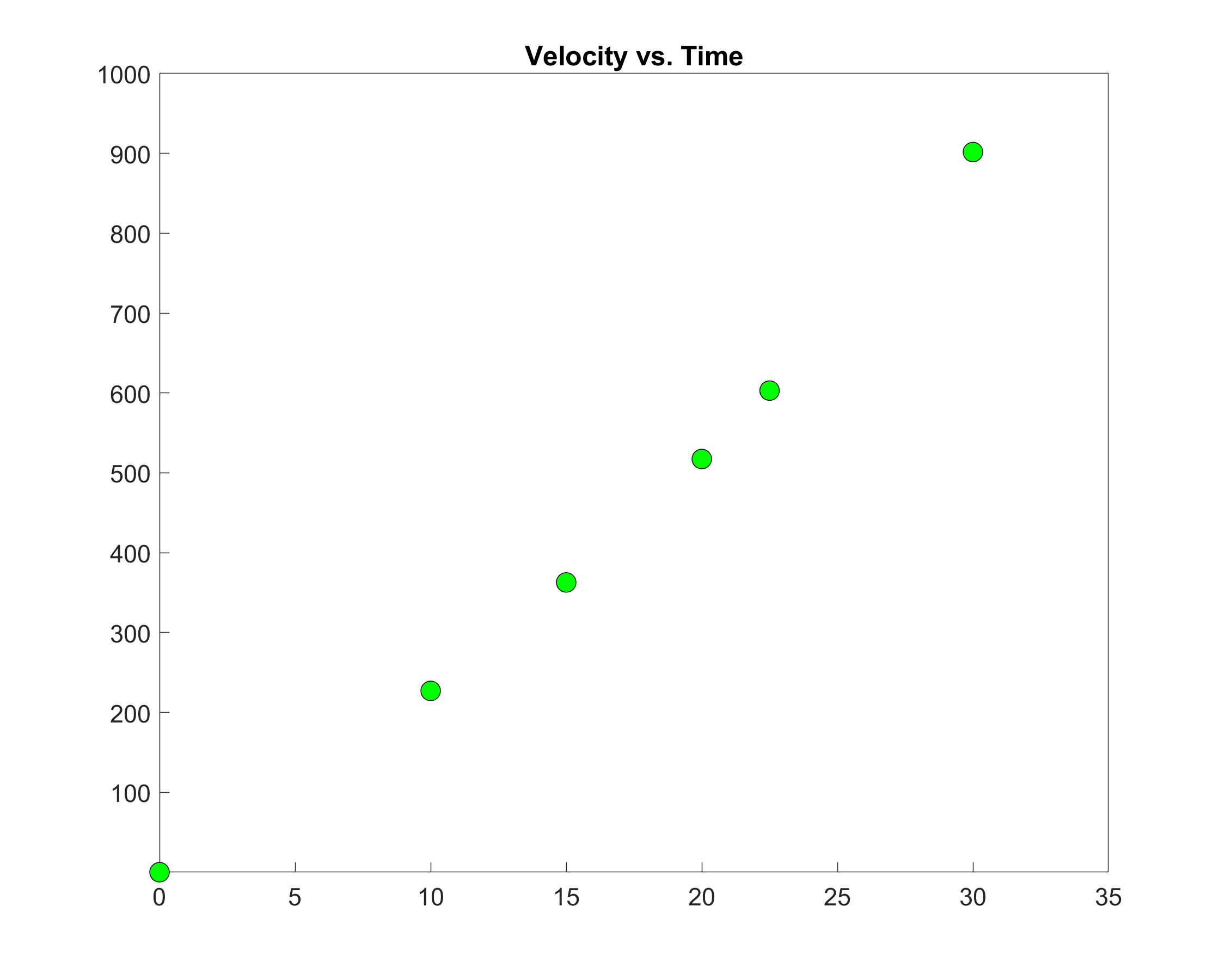
Figure 2. Graph of velocity vs. time data for the rocket example.
Solution
Since we want to evaluate the velocity at \(t = 16\) and use linear spline interpolation, we need to choose the two data points closest to \(t = 16\) that also bracket \(t = 16\) to evaluate it. The two points are \(t_{0} = 15\) and \(t_{1} = 20\).
Then
\[t_{0} = 15,\ v(t_{0}) = 362.78\]
\[t_{1} = 20,\ v(t_{1}) = 517.35\]
gives
\[\begin{split} v(t) &= v(t_{0}) + \frac{v(t_{1}) - v(t_{0})}{t_{1} - t_{0}}(t - t_{0})\\ &= 362.78 + \frac{517.35 - 362.78}{20 - 15}(t - 15)\\ &= 362.78 + 30.913(t - 15),\ 15 \leq t \leq 20 \end{split}\]
At \(t = 16,\)
\[\begin{split} v(16) &= 362.78 + 30.913(16 - 15)\\ &= 393.7 \text{ m/s} \end{split}\]
Linear spline interpolation is no different from linear polynomial interpolation. Linear spline interpolation still uses data only from the two consecutive data points, and data from other points is not used at all. Also, at the interior points of the data, the slope of the spline changes abruptly, which implies that the first derivative is “artificially” not continuous at these points. So how do we overcome these two drawbacks? We can do so by using quadratic or cubic spline interpolation. We discuss these types of spline interpolation in upcoming lessons.
Learning Objectives
After successful completion of this lesson, you should be able to:
1) derive interpolating quadratic spline for discrete data.
Interpolating Quadratic Spline
Quadratic spline interpolation is a method to curve fit data. For quadratic spline interpolation, piecewise quadratics approximates the data between two consecutive data points (Figure 1). Given \(\left( x_{0},y_{0} \right),\left( x_{1},y_{1} \right),......,\left( x_{n - 1},y_{n - 1} \right),\left( x_{n},y_{n} \right)\), fit an interpolating quadratic spline through the data. The quadratics of the spline are given by
\[\begin{split} f(x) &= a_{1}x^{2} + b_{1}x + c_{1},\ x_{0} \leq x \leq x_{1}\\ &= a_{2}x^{2} + b_{2}x + c_{2},\ x_{1} \leq x \leq x_{2}\\ &\ \ \ \ \ \vdots\\ &= a_{n}x^{2} + b_{n}x + c_{n},\ x_{n - 1} \leq x \leq x_{n}\end{split}\]
So how does one find the coefficients of these quadratics? There are \(3n\) such coefficients
\[a_{i},\ i = 1,2,.....,n\]
\[b_{i},\ i = 1,2,.....,n\]
\[c_{i},\ i = 1,2,.....,n\]
To find \(3n\) unknowns, one needs to set up \(3n\) equations and then simultaneously solve them. These \(3n\) equations are found as follows.
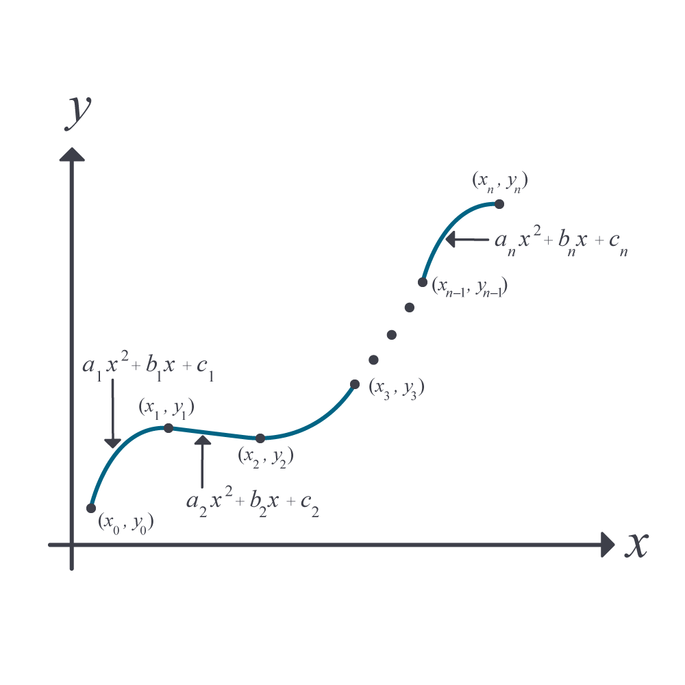
Figure 1. Quadratic spline interpolation
1. Each quadratic goes through two consecutive data points
\[\begin{split} &a_{1}{x_{0}}^{2} + b_{1}x_{0} + c_{1} = f(x_{0})\\ &a_{1}{x_{1}}^{2} + b_{1}x_{1} + c_{1} = f(x_{1})\\ &\vdots\\ &a_{i}{x_{i - 1}}^{2} + b_{i}x_{i - 1} + c_{i} = f(x_{i - 1})\\ &a_{i}{x_{i}}^{2} + b_{i}x_{i} + c_{i} = f(x_{i})\\ \vdots \\ &a_{n}{x_{n - 1}}^{2} + b_{n}x_{n - 1} + c_{n} = f(x_{n - 1})\\ &a_{n}{x_{n}}^{2} + b_{n}x_{n} + c_{n} = f(x_{n}) \end{split}\]
This condition gives \(2n\) equations as there are \(n\) quadratics going through two consecutive data points.
2. The first derivatives of two consecutive quadratics are continuous at the common interior points. For example, the derivative of the first quadratic
\[a_{1}x^{2} + b_{1}x + c_{1}\]
is
\[2a_{1}x + b_{1}\]
The derivative of the second quadratic
\[a_{2}x^{2} + b_{2}x + c_{2}\]
is
\[2a_{2}x + b_{2}\]
and the two are equal at the common interior point \(x = x_{1}\) giving
\[2a_{1}x_{1} + b_{1} = 2a_{2}x_{1} + b_{2}\]
\[2a_{1}x_{1} + b_{1} - 2a_{2}x_{1} - b_{2} = 0\]
Similarly, at the other interior points, \(x_2,\ldots,x_{n-1}\),
\[\begin{split} &2a_{2}x_{2} + b_{2} - 2a_{3}x_{2} - b_{3} = 0\\ \vdots\\ &2a_{i}x_{i} + b_{i} - 2a_{i + 1}x_{i} - b_{i + 1} = 0\\ \vdots \\ &2a_{n - 1}x_{n - 1} + b_{n - 1} - 2a_{n}x_{n - 1} - b_{n} = 0 \end{split}\]
Since there are \((n - 1)\) interior points, we have \((n - 1)\) such equations. So far, the total number of equations obtained is \((2n) + (n - 1) = (3n - 1)\) equations. We still then need one more equation.
We can assume the first quadratic is linear, that is,
\[a_{1} = 0\]
Some assume the last quadratic is linear, that is,
\[a_{n} = 0\]
Others rightly base it on which interval is smaller, \({\lbrack x}_{0},x_{1}\rbrack\) or \({\lbrack x}_{n - 1},x_{n}\rbrack\). If \({|x}_{1} - x_{0}| \leq {|x}_{n} - x_{n - 1}|,\) then one would choose \(a_{1} = 0\), else choose \(a_{n} = 0.\)
This gives us \({3n}\) simultaneous linear equations and \({3n}\) unknowns. These can be solved by several techniques used to solve a general set of simultaneous linear equations.
Learning Objectives
After successful completion of this lesson, you should be able to:
1) conduct quadratic spline interpolation on discrete data,
2) differentiate an interpolating quadratic spline as needed,
3) integrate an interpolating quadratic spline as needed.
Applications
In the previous lesson, you learned the theory of the quadratic spline interpolation method. In this lesson, we apply the theory to given interpolate discrete data to an interpolating quadratic spline.
Example 1
The upward velocity of a rocket is given as a function of time as
Table 1. Velocity as a function of time.
| \(t\ (\text{s})\) | \(v(t)\ (\text{m/s})\) |
|---|---|
| \(0\) | \(0\) |
| \(10\) | \(227.04\) |
| \(15\) | \(362.78\) |
| \(20\) | \(517.35\) |
| \(22.5\) | \(602.97\) |
| \(30\) | \(901.67\) |
a) Determine the value of the velocity at \(t = 16\) seconds using quadratic spline interpolation.
b) Using the interpolating quadratic spline, find the distance covered by the rocket from \(t = 11s\) to \(t = 16s\).
c) Using the interpolating quadratic spline, find the acceleration of the rocket at \(t = 16s\).
Solution
a) Since there are six data points, five quadratics pass through them.
\[\begin{split} v\left( t \right)&= a_{1}t^{2} + b_{1}t + c_{1},\ 0 \leq t \leq 10\\ &= a_{2}t^{2} + b_{2}t + c_{2},\ 10 \leq t \leq 15\\ &= a_{3}t^{2} + b_{3}t + c_{3},\ 15 \leq t \leq 20\\ &= a_{4}t^{2} + b_{4}t + c_{4},\ 20 \leq t \leq 22.5\\ &= a_{5}t^{2} + b_{5}t + c_{5},\ 22.5 \leq t \leq 30 \end{split}\]
The equations are found as follows.
1. Each quadratic passes through two consecutive data points.
Quadratic \(a_{1}t^{2} + b_{1}t + c_{1}\) passes through \(t = 0\) and \(t = 10\).
\[a_{1}{(0)}^{2} + b_{1}\left( 0 \right) + c_{1} = 0 \;\;\;\;\;\;\;\;\;\;\;\; (E1.1)\]
\[a_{1}{(10)}^{2} + b_{1}\left( 10 \right) + c_{1} = 227.04\;\;\;\;\;\;\;\;\;\;\;\; (E1.2)\]
Quadratic \(a_{2}t^{2} + b_{2}t + c_{2}\) passes through \(t = 10\) and \(t = 15\).
\[a_{2}{(10)}^{2} + b_{2}\left( 10 \right) + c_{2} = 227.04\;\;\;\;\;\;\;\;\;\;\;\; (E1.3)\]
\[a_{2}{(15)}^{2} + b_{2}\left( 15 \right) + c_{2} = 362.78\;\;\;\;\;\;\;\;\;\;\;\; (E1.4)\]
Quadratic \(a_{3}t^{2} + b_{3}t + c_{3}\) passes through \(t = 15\) and \(t = 20\).
\[a_{3}{(15)}^{2} + b_{3}\left( 15 \right) + c_{3} = 362.78\;\;\;\;\;\;\;\;\;\;\;\; (E1.5)\]
\[a_{3}{(20)}^{2} + b_{3}\left( 20 \right) + c_{3} = 517.35\;\;\;\;\;\;\;\;\;\;\;\; (E1.6)\]
Quadratic \(a_{4}t^{2} + b_{4}t + c_{4}\)passes through \(t = 20\) and \(t = 22.5\).
\[a_{4}{(20)}^{2} + b_{4}\left( 20 \right) + c_{4} = 517.35\;\;\;\;\;\;\;\;\;\;\;\; (E1.7)\]
\[a_{4}{(22.5)}^{2} + b_{4}\left( 22.5 \right) + c_{4} = 602.97\;\;\;\;\;\;\;\;\;\;\;\; (E1.8)\]
Quadratic \(a_{5}t^{2} + b_{5}t + c_{5}\) passes through \(t = 22.5\) and \(t = 30\).
\[a_{5}{(22.5)}^{2} + b_{5}\left( 22.5 \right) + c_{5} = 602.97\;\;\;\;\;\;\;\;\;\;\;\; (E1.9)\]
\[a_{5}{(30)}^{2} + b_{5}\left( 30 \right) + c_{5} = 901.67\;\;\;\;\;\;\;\;\;\;\;\; (E1.10)\]
2. The quadratics have continuous derivatives at the common interior data points.
At \(t = 10\)
\[2a_{1}\left( 10 \right) + b_{1} - 2a_{2}\left( 10 \right) - b_{2} = 0\;\;\;\;\;\;\;\;\;\;\;\; ((E1.11)\]
At \(t = 15\)
\[2a_{2}\left( 15 \right) + b_{2} - 2a_{3}\left( 15 \right) - b_{3} = 0\;\;\;\;\;\;\;\;\;\;\;\; (E1.12)\]
At \(t = 20\)
\[2a_{3}\left( 20 \right) + b_{3} - 2a_{4}\left( 20 \right) - b_{4} = 0\;\;\;\;\;\;\;\;\;\;\;\; (E1.13)\]
At \(t = 22.5\)
\[2a_{4}\left( 22.5 \right) + b_{4} - 2a_{5}\left( 22.5 \right) - b_{5} = 0\;\;\;\;\;\;\;\;\;\;\;\; (E1.14)\]
3. Assuming the last quadratic \(a_{5}t^{2} + b_{5}t + c_{5}\) is linear (why did we choose the last spline to be linear over the first one?),
\[a_{5} = 0\;\;\;\;\;\;\;\;\;\;\;\; (E1.15)\]
Combining Equations (E1.1) – (E1.15) in matrix form gives
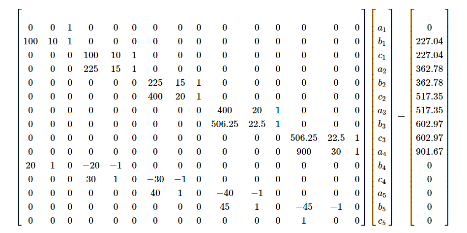
Solving the above \(15\) simultaneous linear equations for the \(15\) unknowns gives
| i | \(a_{i}\) | \(b_{i}\) | \(c_{i}\) |
|---|---|---|---|
| 1 | \(- 0.15667\) | \(24.271\) | \(0\) |
| 2 | \(1.2021\) | \(- 2.9053\) | \(135.88\) |
| 3 | \(- 0.44893\) | \(46.627\) | \(- 235.61\) |
| 4 | \(2.2315\) | \(- 60.589\) | \(836.55\) |
| 5 | \(0\) | \(39.827\) | \(- 293.13\) |
Therefore, the interpolating quadratic spline is given by
\[\begin{split} v\left( t \right) &= - 0.15667t^{2} + 24.271t,\ 0 \leq t \leq 10\\ &= 1.2021t^{2} - 2.9053t + 135.88,\ 10 \leq t \leq 15\\ &= - 0.4489{3t}^{2} + 46.627t - 235.61,\ 15 \leq t \leq 20\\ &= 2.2315t^{2} - 60.589t + 836.55,\ 20 \leq t \leq 22.5\\ &= 39.827t - 293.13,\ 22.5 \leq t \leq 30 \end{split}\;\;\;\;\;\;\;\;\;\;\;\; (E1..16)\]
At \(t = 16\ \text{s}\)
\[\begin{split} v\left( 16 \right) &= - 0.44893\left( 16 \right)^{2} + 46.627(16) - 235.61\\ &= 395.50\ \text{m/s}\end{split}\]
b) The distance covered by the rocket between \(11\ \text{s}\) and \(16\ \text{s}\) seconds can be calculated as
\[s\left( 16 \right) - s\left( 11 \right) = \int_{11}^{16}{v\left( t \right){dt}}\]
But since several quadratics are valid over the limits of integration, we need to break the integral accordingly. Using Equation (E1.16),
\[\begin{split} v\left( t \right) &= 1.2021t^{2} - 2.9053t + 135.88,\ 10 \leq t \leq 15\\ &= - 0.4489{3t}^{2} + 46.627t - 235.61,\ 15 \leq t \leq 20 \end{split}\]
Then
\[\begin{split} s\left( 16 \right) - s\left( 11 \right) &=\int_{11}^{16}v\left( t \right)dt\\ &= \int_{11}^{15}{v\left( t \right)dt + \int_{15}^{16}{v\left( t \right){dt}}} \end{split}\]
Substituting proper quadratics gives
\[\begin{split} s(16) - s(11) &= \int_{11}^{15}{1.2021t^{2} - 2.9053t + 135.88\ dt}\\ &\ \ \ + \int_{15}^{16}{- 0.4489{3t}^{2} + 46.627t - 235.61dt}\\ &= \begin{bmatrix} \\ 1.2021\displaystyle\frac{t^{3}}{3} - 2.9053\displaystyle\frac{t^{2}}{2} + 135.88t \\ \\ \end{bmatrix}\begin{matrix} 15 \\ \\ 11 \\ \end{matrix}\\ &\ \ \ + \begin{bmatrix} \\ - 0.44893\displaystyle\frac{t^{3}}{3} + 46.627\frac{t^{2}}{2} - 235.61t \\ \\ \end{bmatrix}\begin{matrix} 16 \\ \\ 15 \\ \end{matrix}\\ &= 1211.49 + 379.22\\ &= 1590.7\ \text{m} \end{split}\]
c) What is the acceleration at \(t = 16\ \text{s}\)?
\[a\left( 16 \right) = \left.\frac{dv}{{dt}}\right|_{t = 16}\]
Here we use the third quadratic from Equation (E1.15)
\[- 0.4489{3t}^{2} + 46.627t - 235.61,\ 15 \leq t \leq 20\]
as \(t=16\) is in the domain of \(15 \leq t \leq 20.\)
So
\[\begin{split} a\left( t \right) &= \frac{d}{{dt}}v\left( t \right)\\ &= \frac{d}{{dt}}\left( - 0.44893t^{2} + 46.627t - 235.61 \right)\\ &=- 0.89786t + 46.627,\ 15 \leq t \leq 20 \end{split}\]
Hence
\[\begin{split} a\left( 16 \right) &= - 0.89786\left( 16 \right) + 46.627\\ &= 32.261 \ \text{m/s}^2 \end{split}\]
Learning Objectives
After successful completion of this lesson, you should be able to:
1) outline the derivation of cubic spline interpolation.
Introduction
Just like quadratic spline interpolation, cubic spline interpolation is a method to curve fit data. The cubic spline interpolation is the most common degree of spline used.
Interpolating Cubic Spline
Given \(n+1\) data points, \((x_0,y_0),\ (x_1,y_1),\ldots,\ (x_n,y_n),\) fit an interpolating cubic spline through the data. For cubic spline interpolation, piecewise cubic polynomials approximate the data between two consecutive points. The interpolating cubic spline is given by the cubics as
\[\begin{split} f(x) &= a_1x^3 + b_1x^2 + c_1x + d_1,\ x_0\leq x \leq x_1\\ &=a_2x^3 + b_2x^2 + c_2x + d_2,\ x_1\leq x \leq x_2\\ &\ \ \ \ \ \vdots \\ &=a_nx^3 + b_nx^2 + c_nx + d_n,\ x_{n-1}\leq x \leq x_n \end{split}\]
So, how does one find the coefficients of these cubics? There are \(4n\) such coefficients as given below.
\[\begin{split} a_i,\ i &= 1,\ 2,\,\ldots,\ n\\ b_i,\ i &= 1,\ 2,\,\ldots,\ n\\ c_i,\ i &= 1,\ 2,\,\ldots,\ n\\ d_i,\ i &= 1,\ 2,\,\ldots,\ n \end{split}\]
To find the \(4n\) unknowns, we need to set up \(4n\) simultaneous linear equations. The outline of setting up these equations is as follows. We have \(n+1\) data points. Out of these \(n+1\) points, two are the exterior (end) data points, while there are \(((n+1)-2=n-1)\) interior data points.
1. Each cubic must go through two consecutive points. Since we have \(n\) splines, we will get \(2n\) equations.
2. The first derivative of two consecutive cubics is continuous at the common interior data point. Since we have \((n-1)\) interior points, we will get \(2(n-1)\) equations
3. The second derivative of two consecutive cubics is continuous at the common interior data point. Since we have \((n-1)\) interior points, we will get \(2(n-1)\) equations
So far, we have outlined that
\[\begin{split} &(2n) +(n-1) + (n-1)\\ &=4n-2 \end{split}\]
equations can be set up. We need two more equations, and several types of conditions can be used to get them. A few common conditions used are as follows.
1. Assume that the first and last cubic splines are quadratics (\(a_1=0\) and \(a_n=0\)) to get the two more equations. This assumption is called the quadratic end condition.
2. Assume the second derivative of the first and last cubic spline is zero \((6a_1x_0 + 2b_1=0 \ \text{and}\ 6a_nx_n + 2b_n=0)\) at the respective exterior points to get the two more equations. This assumption is called the natural end condition.
Multiple Choice Test
(1). The following n data points, \(\left( x_{1},y_{1} \right)\), \(\left( x_{2},y_{2} \right)\), …….. \(\left( x_{n},y_{n} \right)\), are given. For conducting
quadratic spline interpolation, the \(x\)-data needs to be
(A) equally spaced
(B) placed in ascending or descending order of \(x\) -values
(C) integers
(D) positive
(2). In cubic spline interpolation,
(A) the first derivatives of the cubics are continuous at the interior data points
(B) the second derivatives of the cubics are continuous at the interior data points
(C) the first and the second derivatives of the cubics are continuous at the interior data points
(D) the third derivatives of the cubics are continuous at the interior data points
(3). The following incomplete \(y\) vs. \(x\) data is given.
| \(x\) | \(1\) | \(2\) | \(4\) | \(6\) | \(7\) |
|---|---|---|---|---|---|
| \(y\) | \(5\) | \(11\) | \(????\) | \(????\) | \(32\) |
The data is fit by interpolating quadratic splines given by
\[\begin{split} f\left( x \right) &= ax - 1, \ 1 \leq x \leq 2\\ &= - 2x^{2} + 14x - 9,\ 2 \leq x \leq 4\\ &= bx^{2} + cx + d,\ 4 \leq x \leq 6\end{split}\]
\[= 25x^{2} - 303x + 928,{\ \ \ \ }6 \leq x \leq 7\] where \(a,b,c,\text{and }d\) are constants. The value of \(c\) is most nearly
(A) \(-303.00\)
(B) \(-144.50\)
(C) \(0.0000\)
(D) \(14.000\)
(4). The following incomplete \(y\) vs. \(x\) data is given.
| \(x\) | \(1\) | \(2\) | \(4\) | \(6\) | \(7\) |
|---|---|---|---|---|---|
| \(y\) | \(5\) | \(11\) | \(????\) | \(????\) | \(32\) |
The data is fit by interpolating quadratic spline given by
\[\begin{split} f\left( x \right) &= ax - 1,\ 1 \leq x \leq 2,\\ &= - 2x^{2} + 14x - 9,\ 2 \leq x \leq 4\\ &= bx^{2} + cx + d,\ 4 \leq x \leq 6\\ &= ex^{2} + fx + g,\ 6 \leq x \leq 7\end{split}\]
where \(a,b,c,d,e,f,\text{and }g\) are constants. The value of \(\displaystyle \frac{df}{dx}\) at \(x = 2.6\) most nearly is
(A) \(- 144.50\)
(B) \(- 4.0000\)
(C) \(3.6000\)
(D) \(12.200\)
(5). The following incomplete \(y\) vs. \(x\) data is given.
| \(x\) | \(1\) | \(2\) | \(4\) | \(6\) | \(7\) |
|---|---|---|---|---|---|
| \(y\) | \(5\) | \(11\) | \(????\) | \(????\) | \(32\) |
The data is fit by interpolating quadratic spline given by
\[\begin{split} f\left( x \right) &= ax - 1,\ 1 \leq x \leq 2,\\ &= - 2x^{2} + 14x - 9,\ 2 \leq x \leq 4\\ &= bx^{2} + cx + d,\ 4 \leq x \leq 6\\ &= 25x^{2} - 303x + 928,\ 6 \leq x \leq 7 \end{split}\]
where \(a,b,c,\) and \(d\) are constants. What is the estimated value of \(\displaystyle \int_{1.5}^{3.5}{f\left( x \right){dx}}\)?
(A) \(23.500\)
(B) \(25.667\)
(C) \(25.750\)
(D) \(28.000\)
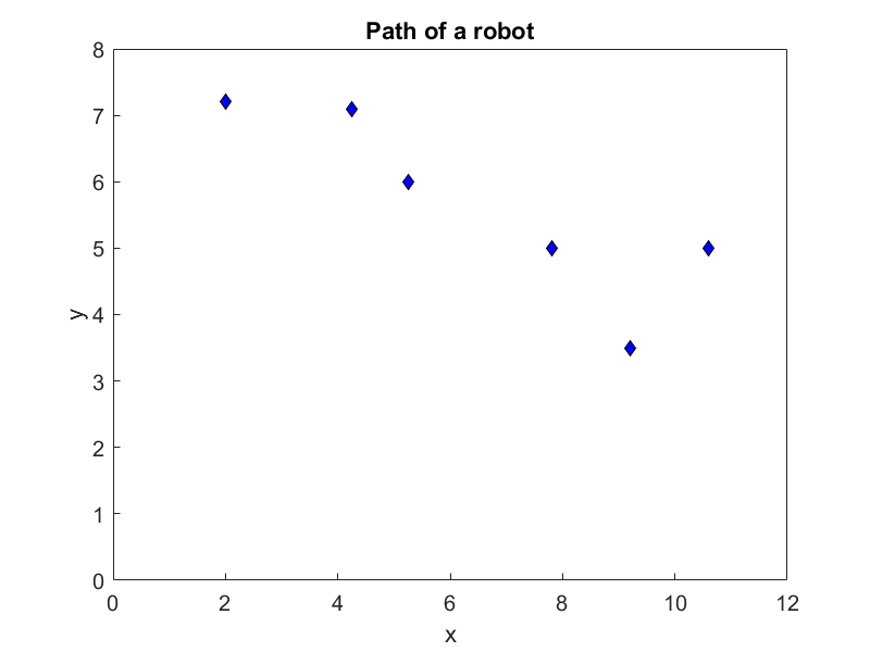
(6). A robot needs to follow a path that passes consecutively through six points, as shown in the
figure. To find the shortest path that is also smooth, you would recommend which of the
following?
(A) Pass a fifth-order polynomial through the data
(B) Pass interpolating linear spline through the data
(C) Pass interpolating quadratic spline through the data
(D) Regress the data to a second-order polynomial
For complete solution, go to
http://nm.mathforcollege.com/mcquizzes/05inp/quiz_05inp_spline_solution.pdf
Problem Set
(1). The following \(y\text{ vs }x\) data is given.
| \(x\) | \(2\) | \(3\) | \(6\) |
|---|---|---|---|
| \(y\) | \(4.75\) | \(5.25\) | \(45\) |
a) Set up the equations to solve for the interpolating quadratic spline that goes through the data.
b) Use a program such as MATLAB to solve the equations and then write down the interpolating quadratic spline.
c) Estimate the value of \(y(3.6)\).
Answer: \(a)\ \left[\begin{matrix}4&2&1&0&0&0\\9&3&1&0&0&0\\0&0&0&9&3&1\\0&0&0&36&6&1\\6&1&0&-6&-1&0\\1&0&0&0&0&0\\\end{matrix}\right]\left[\begin{matrix}a_1\\b_1\\c_1\\a_2\\b_2\\c_2\\\end{matrix}\right]=\left[\begin{matrix}4.75\\5.25\\5.25\\45\\0\\0\\\end{matrix}\right]\)
\(b)\)
| \(i\) | \(a_i\) | \(b_i\) | \(c_i\) |
|---|---|---|---|
| \(1\) | \(0\) | \(0.5\) | \(3.75\) |
| \(2\) | \(4.25\) | \(-25\) | \(42\) |
\(c)\ 7.08\)
(2). The following \(y\ \text{vs}\ x\) data is given.
| \(x\) | \(1\) | \(2\) | \(3\) | \(5\) | \(6\) |
|---|---|---|---|---|---|
| \(y\) | \(4.75\) | \(4\) | \(5.25\) | \(15\) | \(45\) |
The data is fit by interpolating quadratic spline given by
\[\begin{split} f(x) &= - 0.75x + 5.5, 1 \leq x \leq 2\\ &= 2x^{2} - 8.75x + 13.5, 2 \leq x \leq 3\\ &= cx^{2} + gx + h, 3 \leq x \leq 5\\ &= jx^{2} + kx + l, 5 \leq x \leq 6 \end{split}\]
where \(c,\ g,\ h,\ j,\ k,\text{ and } l\) are constants.
a) Find the value of \(c,\ g,\ h,\ j,\ k,\text{ and }l\).
b) Compare the value of the function at \(x = 2.3\) using interpolating linear spline and interpolating quadratic spline.
Answer:
\(a)\) \(c=0.8125\)
\(g=-1.625\)
\(h=2.8125\)
\(j=23.5\)
\(k=-228.5\)
\(l=570\)
\(b)\ \text{linear}= 4.375;\ \text{quadratic}=3.955\)
(3). The following incomplete \(y\) vs. \(x\) data is given.
| \(x\) | \(1\) | \(2.2\) | \(3.7\) | \(5.1\) | \(6\) |
|---|---|---|---|---|---|
| \(y\) | \(4.25\) | \(6\) | \(5.25\) | \(15.1\) | \(?????\) |
The data is fit by interpolating quadratic spline given by
\[\begin{split} f(x) &= 1.4583x + 2.7917, 1 \leq x \leq 2.2\\ &= - 1.3056x^{2} + 7.2028x - 3.5278, 2.2 \leq x \leq 3.7\\ &= cx^{2} + gx + h, 3.7 \leq x \leq 5.1\\ &= jx^{2} + kx + 1, 5.1 \leq x \leq 6 \end{split}\]
where \(c,\ g,\ h,\ j,\ k,\text{ and }l\) are constants. What is the value of \(g\)? Show all your steps clearly.
Answer: \(g=-52.6391\)
(4). The following incomplete \(y\) vs. \(x\) data is given.
| \(x\) | \(1\) | \(2.2\) | \(3.7\) | \(5.1\) | \(6\) |
|---|---|---|---|---|---|
| \(y\) | \(4.25\) | \(6\) | \(5.25\) | \(????\) | \(?????\) |
The data is fit by interpolating quadratic spline given by
\[\begin{split} f(x) &= 1.4583x + 2.7917, 1 \leq x \leq 2.2\\ &= - 1.3056x^{2} + 7.2028x - 3.5272, 2.2 \leq x \leq 3.7\\ &= cx^{2} + gx + h , 3.7 \leq x \leq 5.1\\ &= jx^{2} + kx + l, 5.1 \leq x \leq 6 \end{split}\]
where \(c,\ g,\ h,\ j,\ k,\text{ and }l\) are constants. What is the value of \(\displaystyle \frac{{df}}{{dx}}\) at \(x = 2.67\)?
Answer: \(0.23133\)
(5). The following incomplete \(y\) vs. \(x\) data is given.
| \(x\) | \(1\) | \(2.2\) | \(3.7\) | \(5.1\) | \(6\) |
|---|---|---|---|---|---|
| \(y\) | \(4.25\) | \(6\) | \(5.25\) | \(????\) | \(?????\) |
The data is fit by interpolating quadratic spline given by
\[\begin{split} f(x) &= 1.4583x + 2.7917, 1 \leq x \leq 2.2\\ &= - 1.3056x^{2} + 7.2028x - 3.5272, 2.2 \leq x \leq 3.7\\ &= cx^{2} + gx + h, 3.7 \leq x \leq 5.1\\ &= jx^{2} + kx + l, 5.1 \leq x \leq 6 \end{split}\]
where \(c,\ g,\ h,\ j,\ k,\text{ and }l\) are constants. What is the value of\(\displaystyle\int_{1.5}^{2.5}{f(x)dx}\)?
Answer: \(5.6965\)
(6). Given three data points \((1,6),\ (3,28)\), and \((10, 231)\), it is found that the function \(y = 2x^{2} + 3x + 1\) passes through the three data points. To find the length of the polynomial curve from \(x = 5\) to \(x = 8\), a student uses the formula, \(S = \int_{a}^{b}\sqrt{1 + (dy/dx)^{2}}{dx}\). However, this formula gives the student an integral that cannot be solved exactly. Instead, the student approximates the polynomial curve by drawing interpolating linear spline that consists of piecewise functions from \(x = 5\) to \(x = 6\), from \(x = 6\) to \(x = 7\) and from \(x = 7\) to \(x = 8\). The student then finds the length of the interpolating linear spline from \(x = 5\) to \(x = 8\). What is the student’s estimate of the length of the function from \(x = 5\) to \(x = 8\)?
Answer: \(87.052 \ \text{(getting 87 as the answer is wrong)}\)