Chapter 01.01: Introduction to Numerical Methods
Learning Objectives
After successful completion of this lesson, you should be able to:
1) Enumerate the need for numerical methods.
Introduction
Numerical methods are techniques to approximate mathematical processes (examples of mathematical processes are integrals, differential equations, nonlinear equations).
Approximations are needed because
1) we cannot solve the procedure analytically, such as the standard normal cumulative distribution function
\[\Phi(x) = \frac{1}{\sqrt{2\pi}}\int_{- \infty}^{x}e^{- t^{2}/2}{dt} \;\;\;\;\;\;\;\;\;\;\;\;(1)\]
or
2) the analytical method is intractable, such as solving a set of a thousand simultaneous linear equations for a thousand unknowns for finding forces in a truss (Figure 1).
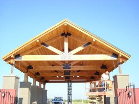
Figure 1. A truss holding a roof.
In the case of Equation (1), an exact solution is not available for \(\Phi(x)\) other than for \(x = 0\) and \(x \rightarrow \infty\). For other values of \(x\) where an exact solution is not available, one may solve the problem by using approximate techniques such as the left-hand Reimann sum you were introduced to in the Integral Calculus course.
In the truss problem, one can solve \(1000\) simultaneous linear equations for \(1000\) unknowns without using a calculator. One can use fractions, long divisions, and long multiplications to get the exact answer. But just the thought of such a task is laborious. The task may seem less laborious if we are allowed to use a calculator, but it would still fall under the category of an intractable, if not an impossible, problem. So, we need to find a numerical technique and convert it into a computer program that solves a set of \(n\) equations and \(n\) unknowns.
Again, what are numerical methods? They are techniques to solve a mathematical problem approximately. As we go through the course, you will see that numerical methods let us find solutions close to the exact one, and we can quantify the approximate error associated with the answer. After all, what good is an approximation without quantifying how good the approximation is?
Learning Objectives
After successful completion of this lesson, you should be able to:
1) go through the stages (problem description, mathematical modeling, solving and implementation) of solving a particular physical problem.
Introduction
Numerical methods are used by engineers and scientists to solve problems. However, numerical methods are just one step in solving an engineering problem. There are four steps for solving an engineering problem, as shown in Figure 1.
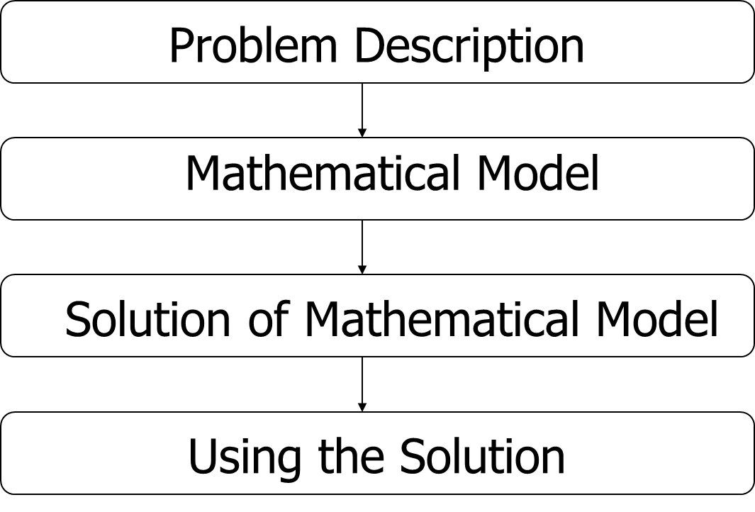
Figure 1 Steps of solving a problem
The first step is to describe the problem. The description would involve writing the background of the problem and the need for its solution. The second step is developing a mathematical model for the problem, and this could include the use of experiments or/and theory. The third step involves solving the mathematical model. The solution may consist of analytical or/and numerical means. The fourth step is implementing the solution to see if the problem is solved.
Let us see through an example of these four steps of solving an engineering problem.
Problem Description
To make the fulcrum (Figure 2) of a bascule bridge, a long hollow steel shaft called the trunnion is shrink fit into a steel hub. The resulting steel trunnion-hub assembly is then shrunk-fit into the girder of the bridge.
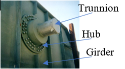
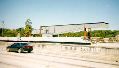
Figure 2 Trunnion-Hub-Girder (THG) assembly.
The shrink-fitting is done by first immersing the trunnion in a cold medium such as a dry-ice/alcohol mixture. After the trunnion reaches the steady-state temperature, that is, the temperature of the cold medium, the outer diameter of the trunnion contracts. The trunnion is taken out of the medium and slid through the hole of the hub (Figure 3).

Figure 3 Trunnion slided through the hub after contracting
When the trunnion heats up, it expands and creates an interference fit with the hub. In 1995, on one of the bridges in Florida, this assembly procedure did not work as designed. Before the trunnion could be inserted fully into the hub, the trunnion got stuck. Luckily, the trunnion was taken out before it got stuck permanently. Otherwise, a new trunnion and hub would need to be ordered at the cost of \(\$50,000\). Coupled with construction delays, the total loss could have been more than a hundred thousand dollars.
Why did the trunnion get stuck - because the trunnion had not contracted enough to slide through the hole. Can you find out why?
Simple Mathematical Model
A hollow trunnion of an outside diameter \(12.363^{\prime\prime}\) is to be fitted in a hub of inner diameter \(12.358^{\prime\prime}\). The trunnion was put in a dry ice/alcohol mixture (temperature of the fluid - dry-ice/alcohol mixture is \(- 108{^\circ}\text{F}\)) to contract the trunnion so that it can be slid through the hole of the hub. To slide the trunnion without sticking, a diametrical clearance of at least \(0.01^{\prime\prime}\) is required between the trunnion and the hub. Assuming the room temperature is \(80{^\circ}\text{F}\), is immersing the trunnion in a dry-ice/alcohol mixture a correct decision?
To calculate the contraction in the diameter of the trunnion, the thermal expansion coefficient at room temperature is used. In that case, the reduction \(\Delta D\) in the outer diameter of the trunnion is
\[\displaystyle\Delta D = D\alpha\Delta T \;\;\;\;\;\;\;\;\;\;\;\; (1)\]
where
\[D = \text{ outer diameter of the trunnion,}\]
\[\alpha = \text{ coefficient of thermal expansion coefficient at room temperature, and}\]
\[\Delta T = \text{change in temperature.}\]
Solution to Simple Mathematical Model
Given
\[D = 12.363^{\prime\prime}\]
\[\alpha = 6.47 \times 10^{-6}\ \text{in/in/}^{\circ}\text{F} \text{ at } 80{^\circ}\text{F}\]
\[\displaystyle \begin{split} \Delta T&= T_{{fluid}} - T_{{room}}\\ &= - 108 - 80\\ &= - 188{^\circ}\ \text{F}\end{split}\]
where
\[T_{{fluid}}= \text{ temperature of dry-ice/alcohol mixture}\]
\[T_{{room}}= \text{ room temperature}\]
the reduction in the outer diameter of the trunnion from Equation (1) hence is given by
\[\begin{split} \Delta D &= (12.363)\left( 6.47 \times 10^{- 6} \right)\left( - 188 \right)\\ &=- 0.01504^{\prime\prime} \end{split}\]
So the trunnion is predicted to reduce in diameter by \(0.01504^{\prime\prime}\). But is this enough reduction in diameter? As per specifications, the trunnion diameter needs to change by
\[ \begin{split} &= \text{trunnion outside diameter} - \text{hub inner diameter} + \text{diametric clearance}\\ &= 12.363 - 12.358 + 0.01\\ &= - 0.015^{\prime\prime} \end{split}\]
So, according to his calculations, immersing the steel trunnion in dry-ice/alcohol mixture gives the desired contraction of greater than \(0.015^{\prime\prime}\) as the predicted contraction is \(0.01504^{\prime\prime}\). But, when the steel trunnion was put in the hub, it got stuck. Why did this happen? Was our mathematical model adequate for this problem, or did we create a mathematical error?
Accurate Mathematical Model
As shown in Figure 4 and Table 1, the thermal expansion coefficient of steel decreases with temperature and is not constant over the range of temperature the trunnion goes through. Hence, Equation (1) would overestimate the thermal contraction.
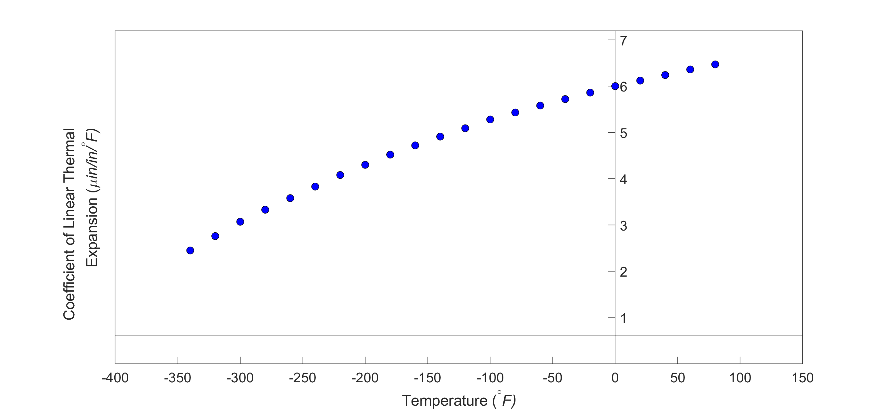
Figure 4 Varying thermal expansion coefficient as a function of temperature for cast steel.
The contraction in the diameter of the trunnion for which the thermal expansion coefficient varies as a function of temperature is given by
\[ \Delta D = D\int_{T_{room}}^{T_{fluid}} \alpha dT \;\;\;\;\;\;\;\;\;\;\;\; (2)\]
Solution to More Accurate Mathematical Model
So, one needs to curve fit the data to find the coefficient of thermal expansion as a function of temperature. This curve is found by regression where we best fit a function to the data given in Table 1. In this case, we may fit a second-order polynomial
\[\displaystyle\alpha = a_{0} + a_{1} T + a_{2} T^{2}\;\;\;\;\;\;\;\;\;\;\;\; (3)\]
Table 1 Instantaneous thermal expansion coefficient as a function of temperature.
| Temperature | Instantaneous Thermal Expansion |
|---|---|
| \({^\circ}\text{F}\) | \(\mu \text{in/in/}^{\circ}\text{F}\) |
| \(80\) | \(6.47\) |
| \(60\) | \(6.36\) |
| \(40\) | \(6.24\) |
| \(20\) | \(6.12\) |
| \(0\) | \(6.00\) |
| \(-20\) | \(5.86\) |
| \(-40\) | \(5.72\) |
| \(-60\) | \(5.58\) |
| \(-80\) | \(5.43\) |
| \(-100\) | \(5.28\) |
| \(-120\) | \(5.09\) |
| \(-140\) | \(4.91\) |
| \(-160\) | \(4.72\) |
| \(-180\) | \(4.52\) |
| \(-200\) | \(4.30\) |
| \(-220\) | \(4.08\) |
| \(-240\) | \(3.83\) |
| \(-260\) | \(3.58\) |
| \(-280\) | \(3.33\) |
| \(-300\) | \(3.07\) |
| \(-320\) | \(2.76\) |
| \(-340\) | \(2.45\) |
The values of the coefficients in the above Equation (3) will be found by polynomial regression (we will learn how to do this later in the chapter on Nonlinear Regression). At this point, we are just going to give you these values, and they are
\[\begin{bmatrix} a_{0} \\ a_{1} \\ a_{2} \\ \end{bmatrix} = \begin{bmatrix} 6.0150 \times 10^{- 6} \\ 6.1946 \times 10^{- 9} \\ - 1.2278 \times 10^{- 11} \\ \end{bmatrix}\]
to give the polynomial regression model (Figure 5) as
\[\displaystyle \begin{split} \alpha &= a_{0} + a_{1}T + a_{2}T^{2}\\ &= {6.0150} \times {1}{0}^{- 6} + {6.1946} \times {1}{0}^{- 9}T - {1.2278} \times {1}{0}^{- {11}}T^{2} \end{split} \;\;\;\;\;\;\;\;\;\;\;\; (4)\]
Knowing the values of \(a_{0}\), \(a_{1}\), and \(a_{2}\), we can then find the contraction in the trunnion diameter from Equations (2) and (3) as
\[\begin{split} \displaystyle\Delta D &= D\int_{T_{{room}}}^{T_{{fluid}}}{(a_{0} + a_{1}T + a_{2}T^{2}}){dT}\\ &= D\left\lbrack a_{0}T + a_{1}\frac{T^{2}}{2} + a_{2}\frac{T^{3}}{3} \right\rbrack\begin{matrix} T_{{fluid}} \\ \\ T_{{room}} \\ \end{matrix}\\ &= D\lbrack a_{0}(T_{{fluid}} - T_{{room}}) + a_{1}\frac{({T_{{fluid}}}^{2} - {T_{{room}}}^{2})}{2}\\ & \ \ \ \ \ + a_{2}\frac{({T_{{fluid}}}^{3} - {T_{{room}}}^{3})}{3}\rbrack\;\;\;\;\;\;\;\;\;\;\;\;(5) \end{split}\]
Substituting the values of the variables gives
\[\displaystyle \begin{split} \Delta D &= 12.363\begin{bmatrix} 6.0150 \times 10^{- 6} \times ( - 108 - 80) \\ + 6.1946 \times 10^{- 9}\displaystyle \frac{\left( ( - 108)^{2} - (80)^{2} \right)}{2} \\ - 1.2278 \times 10^{- 11}\displaystyle \frac{(( - 108)^{3} - (80)^{3})}{3} \\ \end{bmatrix}\\ &= - 0.013689^{\prime\prime}\end{split}\]
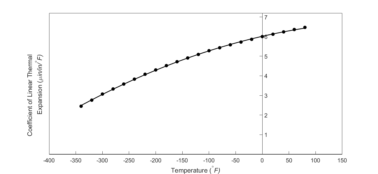
Figure 5 Second-order polynomial regression model for the coefficient of thermal expansion as a function of temperature.
What do we find here? The contraction in the trunnion is not enough to meet the required specification of \(0.015^{\prime\prime}\).
Implementing the Solution
Although we were able to find out why the trunnion got stuck in the hub, we still need to find and implement a solution. What if the trunnion were immersed in a medium that was cooler than the dry-ice/alcohol mixture of \(- 108{^\circ}F\) , say liquid nitrogen, which has a boiling temperature of \(- 321{^\circ}F\)? Will that be enough for the specified contraction in the trunnion?
As given in Equation (5)
\[\displaystyle \begin{split} \Delta D &= D\int_{T_{{room}}}^{T_{{fluid}}}{(a_{0} + a_{1}T + a_{2}T^{2}}){dT}\\ &= D\left\lbrack a_{0}T + a_{1}\frac{T^{2}}{2} + a_{2}\frac{T^{3}}{3} \right\rbrack\begin{matrix} T_{{fluid}} \\ \\ T_{{room}} \\ \end{matrix}\\ &= D\lbrack a_{0}(T_{{fluid}} - T_{{room}}) + a_{1}\frac{({T_{{fluid}}}^{2} - {T_{{room}}}^{2})}{2}\\ & \ \ \ \ \ + a_{2}\frac{({T_{{fluid}}}^{3} - {T_{{room}}}^{3})}{3}\rbrack\;\;\;\;\;\;\;\;\;\;\;\; (5-repeated) \end{split}\]
which gives
\[\displaystyle \begin{split} \Delta D &= 12.363\begin{bmatrix} 6.0150 \times 10^{- 6} \times ( - 321 - 80) \\ + 6.1946 \times 10^{- 9} \displaystyle\frac{\left( ( - 321)^{2} - (80)^{2} \right)}{2} \\ \ - 1.2278 \times 10^{- 11} \displaystyle\frac{(( - 321)^{3} - (80)^{3})}{3} \\ \end{bmatrix}\\ &= - 0.024420^{\prime\prime} \end{split}\]
The magnitude of this contraction is larger than the specified value of \(0.015^{\prime\prime}\)
So here are some questions that you may want to ask yourself later in the course?
1) What if the trunnion were immersed in liquid nitrogen (boiling temperature\(= - 321{^\circ}\text{F}\))? Will that cause enough contraction in the trunnion?
2) Rather than regressing the thermal expansion coefficient data to a second-order polynomial so that one can find the contraction in the trunnion OD, how would you use the trapezoidal rule of integration for unequal segments?
3) What is the relative difference between the two results?
4) We chose a second-order polynomial for regression. Would a different order polynomial be a better choice for regression? Is there an optimum order of polynomial we could use?
Learning Objectives
After successful completion of this lesson, you should be able to:
1) enumerate the seven mathematical processes for which numerical methods are used.
Introduction
Numerical methods are techniques to approximate mathematical processes. This introductory numerical methods course will develop and apply numerical techniques for the following mathematical processes:
1) Roots of Nonlinear Equations
2) Simultaneous Linear Equations
3) Curve Fitting via Interpolation
4) Differentiation
5) Curve Fitting via Regression
6) Numerical Integration
7) Ordinary Differential Equations.
Some undergraduate courses in numerical methods may include topics of partial differential equations, optimization, and fast Fourier transforms as well.
Roots of a Nonlinear Equation
The ubiquitous formula
\[ x = \frac{- b \pm \sqrt{b^2 - 4ac}}{2a} \;\;\;\;\;\;\;\;\;\;\;\; (1)\]
of finding the roots of a quadratic equation \(\displaystyle ax^{2} + bx + c = 0\) goes back to the ancient world. But in the real world, we get equations that are not just the quadratic ones. They can be polynomial equations of a higher order and transcendental equations.
Take an example of a floating ball shown in Figure 1, where you are asked to find the depth to which the ball will get submerged when floating in the water.
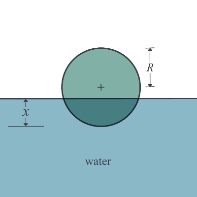
Figure 1. Depth to which a ball is floating
Assume that the ball has a density of \(600\ \text{kg}/\text{m}^{3}\) and has a radius of \(0.055\ \text{m}\). On applying the Newtons laws of motion and hence equating the weight of the ball to the buoyancy force, one finds that the depth, \(x\) in meters, to which the ball is underwater and is given by
\[\displaystyle 3.993 \times 10^{- 4} - 0.165x^{2} + x^{3} = 0 \;\;\;\;\;\;\;\;\;\;\;\; (2)\]
Equation(2) is a cubic equation that you will need to solve. The equation will have three roots, and the root that is between \(0\ \text{m}\) (just touching the water surface) and \(0.11\ \text{m}\) (almost submerged) would be the depth to which the ball is submerged. The two other roots would be physically unacceptable. Note that a cubic equation with real coefficients can have a set of one real root and two complex roots or a set of three real roots. You may wonder why such an application could be important? Let’s suppose you are filling in this tank with water, and you are using this ball as a control so that when the ball goes all the way to the top that the flow of the water stops – say in a fish tank that needs replenishing while the owner is away for a few weeks. So, we do need to figure out how much of the ball is submerged underwater.
A cubic equation can be solved exactly by radicals, but it is a tedious process. The same is true but even more complicated for a general fourth-order polynomial equation as well. However, there is no closed-form solution available for a general polynomial equation of fifth-order or more. So, one has to resort to numerical techniques to solve polynomial and other transcendental nonlinear equations (e.g., finding the nonzero roots of \(\tan x = x\)).
Simultaneous Linear Equations
Ever since you were exposed to algebra, you have been solving simultaneous linear equations.
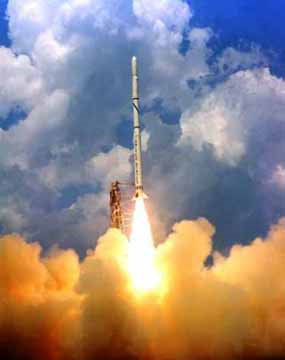
Figure 2. A rocket going upwards
Take this problem statement as an example. Suppose the upward velocity of a rocket (Figure 2) is given at three different times (Table 1).
Table 1: Velocity vs. time data
| Time, t (s) |
Velocity, v (m/s) |
|---|---|
| \(5\) | \(106.8\) |
| \(8\) | \(177.2\) |
| \(12\) | \(600.0\) |
The velocity data is approximated by a polynomial as
\[\displaystyle v\left( t \right) = at^{2} + {bt} + c\ {, 5} \leq t \leq {12}.\;\;\;\;\;\;\;\;\;\;\;\;(3)\]
To estimate the velocity at a time that is not given to us, we can set up the equations to find the coefficients \(a,b,c\) of the velocity profile.
The polynomial in Equation (3) is going through three data points \(\left( t_{1},v_{1} \right),\left( t_{2},v_{2} \right),\) and \(\left( t_{3},v_{3} \right)\) where from Table 1
\[\begin{split} t_{1} &= 5,v_{1} = 106.8\\ t_{2} &= 8,v_{2} = 177.2\\ t_{3} &= 12,v_{3} = 600.0 \end{split}\]
Requiring that \(v\left( t \right) = at^{2} + bt + c\) passes through the three data points, gives
\[\begin{split} v\left( t_{1} \right) &= v_{1} = at_{1}^{2} + bt_{1} + c\\ v\left( t_{2} \right) &= v_{2} = at_{2}^{2} + bt_{2} + c\\ v\left( t_{3} \right) &= v_{3} = at_{3}^{2} + bt_{3} + c \end{split}\]
Substituting the data \(\left( t_{1},\ v_{1} \right),\ \left( t_{2},\ v_{2} \right),\) and \(\left( t_{3},\ v_{3} \right)\) gives
\[\begin{split} a\left( 5^{2} \right) + b\left( 5 \right) + c = 106.8 \\ a\left( 8^{2} \right) + b\left( 8 \right) + c = 177.2 \\ a\left( 12^{2} \right) + b\left( 12 \right) + c = 600.0 \end{split}\]
Or
\[\begin{split} 25a + 5b + c = 106.8 \\ 64a + 8b + c = 177.2 \\ 144a + 12b + c = 600.0 \end{split} \;\;\;\;\;\;\;\;\;\;\;\; (4)\]
Solving a few simultaneous linear equations such as the above set can be done without the knowledge of numerical techniques. However, imagine that instead of three given points, you were given 10 data points. Now the setting up as well as solving the set of 10 simultaneous linear equations without numerical techniques becomes laborious, if not impossible.
Curve Fitting by Interpolation
Interpolation involves that given a function as a set of data points, how does one find the value of the function at points that are not given to us. For this, we choose a function, called an interpolant, and make it pass through all the points involved.
You may think that you have already used interpolation in courses such as Thermodynamics and Statistics. After all, it was just taking two points from a table at the back of the textbook or online and finding the value of the function at a point in between by using a straight line.
Take this problem statement as an example. Let’s suppose the upward velocity of a rocket is given at three different times (Table 1).
If one asked you to estimate the velocity at \(7\ \text{s}\), one might simply use the straight-line formula you are most accustomed to as given below.
Given (\(t_{1},\ v_{1}\)) and (\(t_{2},\ v_{2}\)), the value of the function \(v\) at \(t\) is given by
\[\displaystyle v = v_{1} + \frac{v_{2} - v_{1}}{t_{2} - t_{1}}(t - t_{1}) \;\;\;\;\;\;\;\;\;\;\;\; (5)\]
Although this is possibly enough for courses such as Thermodynamics and Statistics, there are two questions to ask. Is the value calculated accurately, and how accurate is it? To know that, one needs to calculate at least more than one value. In the above example of a rocket velocity vs. time, one can instead use a second-order polynomial interpolant and set up the three equations and three unknowns to find the unknown coefficients, \(a\), \(b\), and \(c\) as given in the previous section.
\[v\left( t \right) = at^{2} + {bt} + c{ ,\ 5} \leq t \leq {12}\;\;\;\;\;\;\;\;\;\;\;\; (6)\]
Then, the resulting second-order polynomial can be used to find the velocity at \(t = 7\ \text{s}\).
The value obtained from the second-order polynomial (Equation (6)) can be considered to be a new measure of the value of \(v( 7)\), and the first-order polynomial (Equation (5)) result can be used to determine the accuracy of the results.
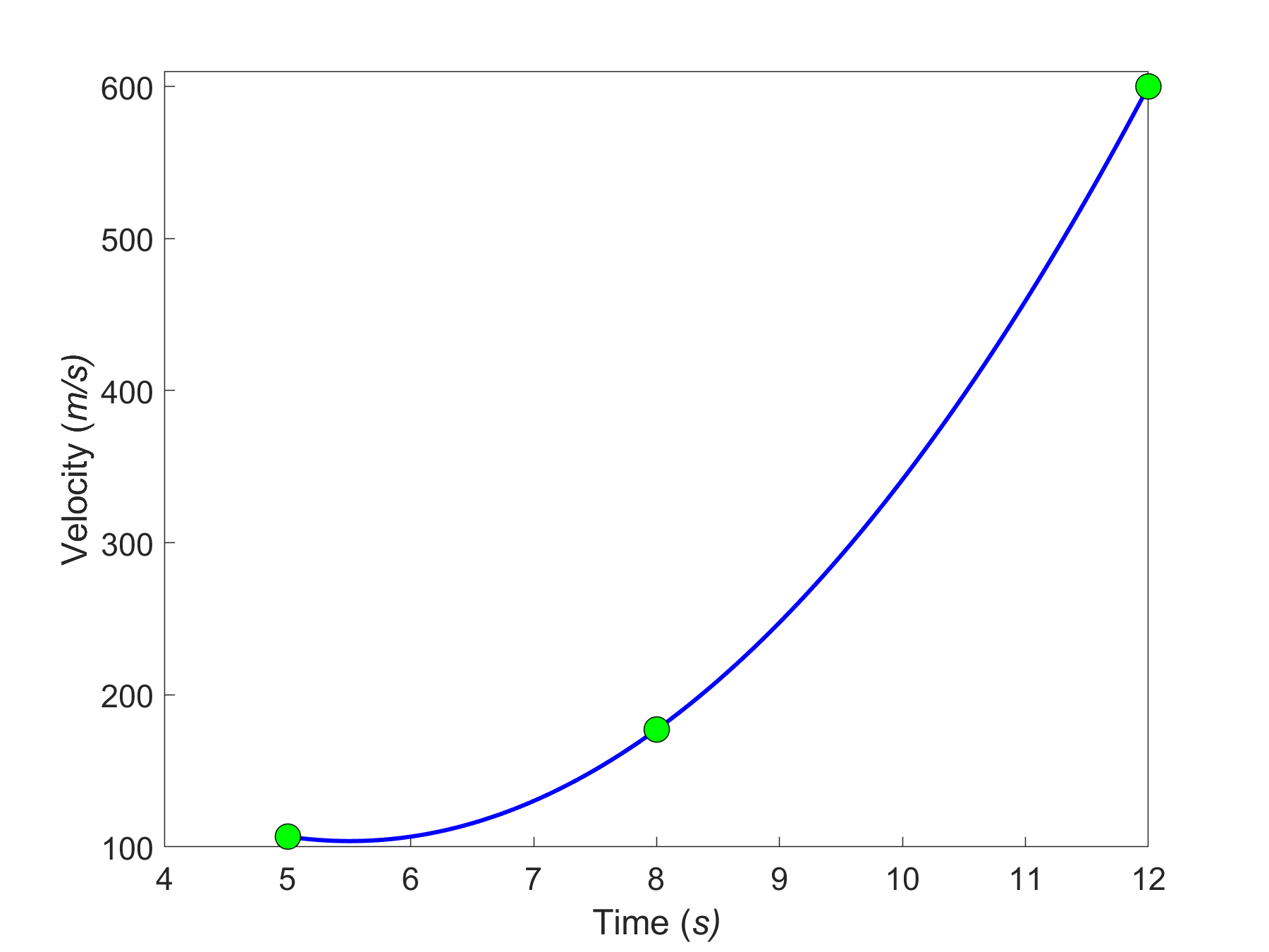
Figure 3. Second-order interpolant for velocity vs. time.
Numerical Differentiation
You have taken a semester-long course in Differential Calculus, where you found derivatives of continuous functions. So let’s suppose somebody gives you the velocity of a rocket as a continuous and at least once differentiable function of time and wants you to find acceleration. Indeed for this particular problem, you can use your differential calculus knowledge to differentiate the velocity function to get the acceleration and put in the value of time, \(t = 7\ \text{s}\). What if the velocity vs. time is not given as a continuous and at least once differentiable function? Instead, let’s say the function is given at discrete data points (Table 1). How are you then going to find out what the acceleration at \(t = 7\ \text{s}\)? Do we draw a straight line from \((5,106.8)\) to \((8,177.2)\) and use the straight-line slope as the estimate of acceleration? How do we know that this is adequate? We could incorporate all three points and find a second-order polynomial as given by Equation (6). This polynomial can now be differentiated to estimate the acceleration at \(t = 7\ \text{s}\). Now the two values can be used to evaluate the accuracy of the calculated acceleration.
Curve Fitting by Regression
When we talked about curve fitting by interpolation, the chosen interpolant needs to go through all the points considered. What happens when we are given many data points, and we instead want a simplified formula to explain the relationship between two variables. See, for example, in Figure 4a, we are given the coefficient of linear thermal expansion data for cast steel as a function of temperature. Looking at the data, one may proclaim that a straight line could explain the data, and that is drawn in Figure 4b. How we draw this straight line is what is called regression. It would be based on minimizing some form of the residuals between what is observed (given data points) and what is predicted (straight line). It does not mean that every time you have data given to you, you draw a straight line. It is possible that a second-order polynomial or a transcendental function other than the first-order polynomial will be a better representation of this particular data. So these are the questions that we will answer when we discuss regression. We will also discuss the adequacy of linear regression models.
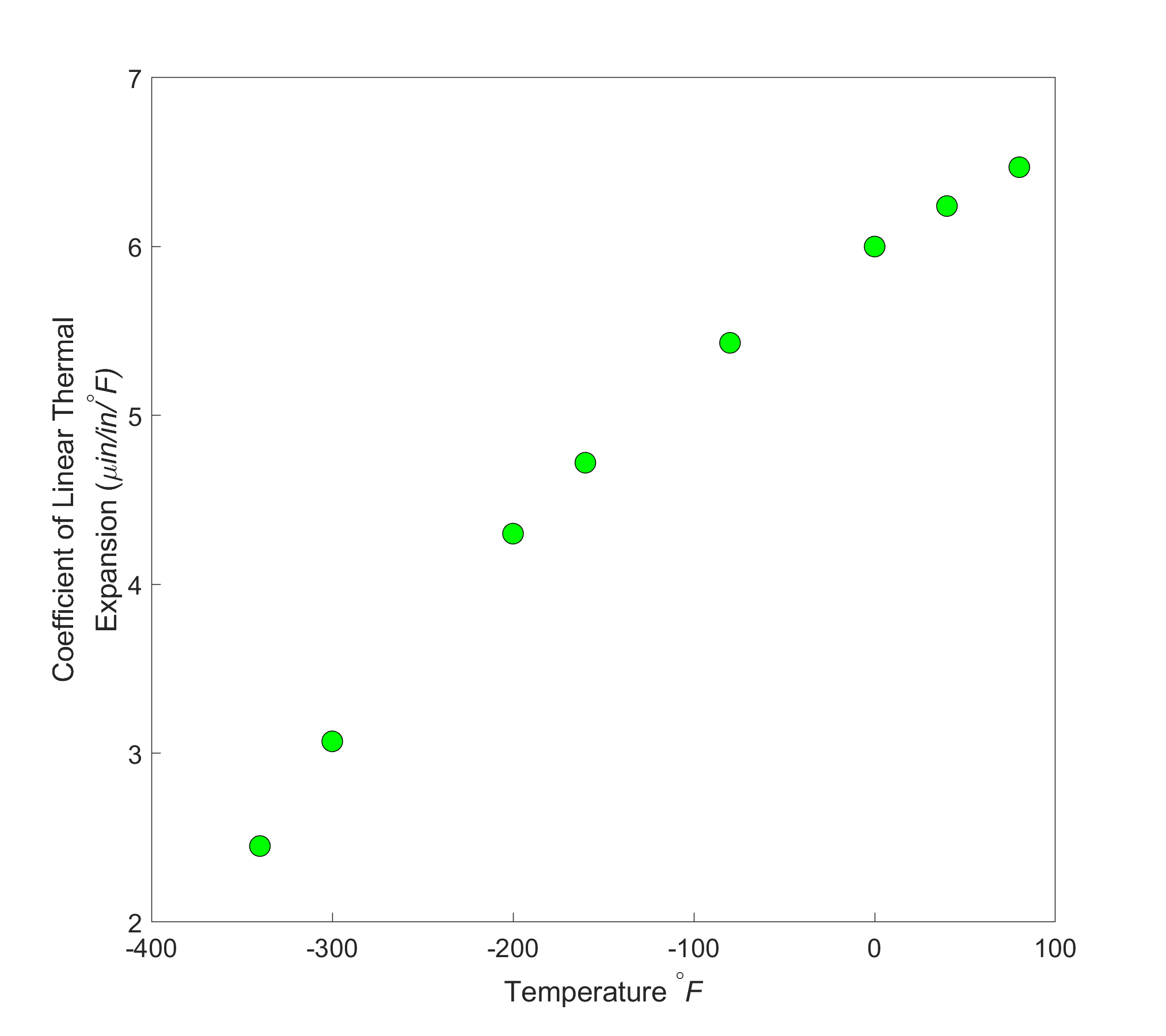
Figure 4a. Coefficient of linear thermal expansion for cast steel as a function of temperature
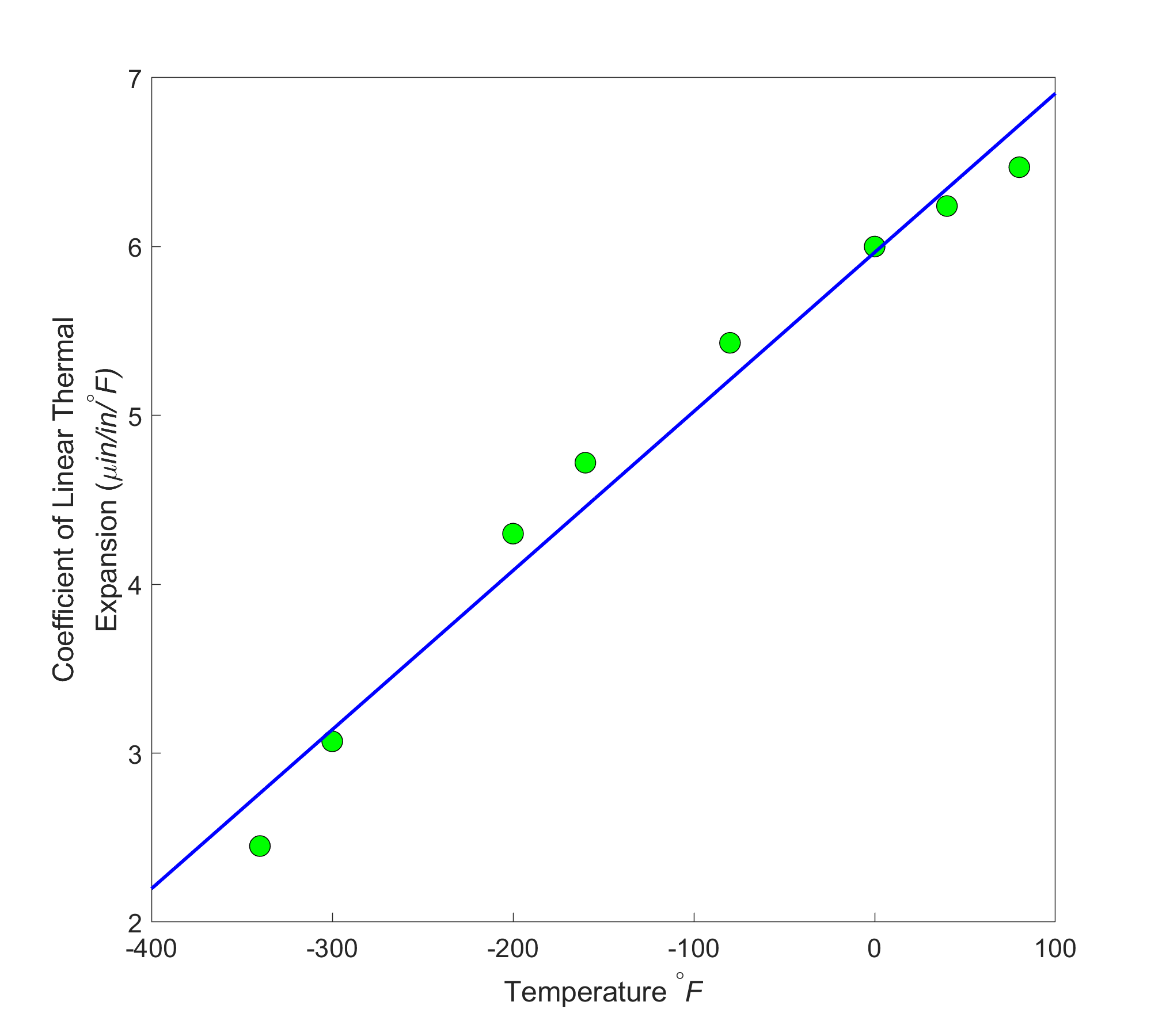
Figure 4b. Linear regression model of coefficient of linear thermal expansion for cast steel as a function of temperature
Numerical Integration
You have taken a whole course on integral calculus. Now, why would we need to make numerical approximations of integrals? Just like the standard normal cumulative distribution function
\[\displaystyle\Phi(x) = \frac{1}{\sqrt{2\pi}}\int_{- \infty}^{x}e^{- t^{2}/2}{dt} \;\;\;\;\;\;\;\;\;\;\;\; (7)\]
cannot be solved exactly, or when the integrand values are given at discrete data points, we need to use numerical methods of integration.
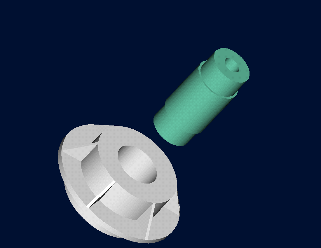
Figure 5. Trunnion of a fulcrum assembly of a bascule bridge
In the previous lesson, we looked at the example of contracting the diameter of a trunnion for a bascule bridge fulcrum assembly by dipping it in a mixture of dry ice and alcohol. The contraction is given by
\[\Delta D = D\int_{T_{room}}^{T_{fluid}}{\alpha\ dT} \;\;\;\;\;\;\;\;\;\;\;\; (8)\]
where
\[D = \text{outer diameter of the trunnion,}\]
\[\alpha = \text{coefficient of linear thermal expansion that is varying with temperature}\]
\[T_{{room}}= \text{room temperature}\]
\[T_{{fluid}}= \text{temperature of dry-ice alcohol mixture.}\]

Figure 6 Varying thermal expansion coefficient as a function of temperature for cast steel.
From Figure 4a, one can note that the coefficient of thermal expansion is only given at discrete temperatures and not as a known continuous function that could be integrated exactly. So we have to resort to numerical methods by approximating the data, say, by a second-order polynomial obtained via regression.
In Figure 6, the thermal expansion coefficient of typical cast steel is approximated by a second-order regression polynomial as given by Equation (9) (how we get this is a later lesson in regression) as
\[\displaystyle\alpha = - 1.2278 \times 10^{- 11}T^{2} + 6.1946 \times 10^{- 9}T + 6.0150 \times 10^{- 6} \;\;\;\;\;\;\;\;\;\;\;\; (9)\]
The contraction of the diameter then is given by
\[\displaystyle\Delta D = D\int_{T_{{room}}}^{T_{{fluid}}}{\left( - 1.2278 \times 10^{- 11}T^{2} + 6.1946 \times 10^{- 9}T + 6.015 \times 10^{- 6} \right){dT}} \;\;\;\;\;\;\;\; (10)\]
and can now be calculated using integral calculus.
Numerical Solution of Ordinary Differential Equations
Taking the same example of the trunnion being dipped in a dry-ice/alcohol mixture, one could ask the question - What would the temperature of the trunnion be after dipping it in the mixture for 30 minutes. The model is given by an ordinary differential equation for the temperature \(\theta\) as a function of time, \({t.}\)
\[\displaystyle- {hA} \left(\theta - \theta_{a} \right) = {mC} \frac{d \theta}{dt}\;\;\;\;\;\;\;\;\;\;\;\; (11)\]
where
\[h= \text{the convective cooling coefficient,}\ \text{W/m}^{2}\text{-K}\]
\[A = \text{surface area},\ \text{m}^2\]
\[\theta_{a} = \text{ambient temperature of dry-ice/alcohol mixture},\ \text{K}\]
\[m = \text{mass of the trunnion, kg}\]
\[C = \text{specific heat of the trunnion,}\ \text{J/(kg-K)}\]
The differential Equation (11) can be solved exactly by using the classical solution, Laplace transform, or separation of variables techniques. So, where do numerical methods enter into the picture for this problem? For the temperature range of room temperatures to cold media such as dry-ice/alcohol, several of the variables in Equation (11) are not constant but change with the temperature. These include the convection coefficient \(h\) as well as the specific heat \(C\). Now, this differential equation has turned nonlinear as follows.
\[\displaystyle- h(\theta)A\left( \theta - \theta_{a} \right) = mC(\theta)\frac{{d \theta }}{{dt}} \;\;\;\;\;\;\;\;\;\;\;\; (12)\]
The ordinary differential Equation (12) cannot be solved by exact methods and would need to be solved by a numerical method.
In the above discussion, we have illustrated the need for numerical methods for each of the seven mathematical processes in the course. In the lessons to follow, we will be developing various numerical techniques to approximate the mathematical processes to calculate acceptable accurate values while calculating associated errors.
Multiple Choice Test
(1). Solving an engineering problem requires four steps. In order of sequence, the four steps are
(A) formulate, model, solve, implement
(B) formulate, solve, model, implement
(C) formulate, model, implement, solve
(D) model, formulate, implement, solve
(2). One of the roots of the equation \(x^{3} - 3x^{2} + x - 3 = 0\) is
(A) \(-1\)
(B) \(1\)
(C) \(\sqrt{3}\)
(D) \(3\)
(3). The solution to the set of equations
\[\begin{split} 25a + b + c &= 25 \\ 64a + 8b + c &= 71\\ 144a + 12b + c &= 155 \end{split}\]
most nearly is \(\left( a,b,c \right) =\)
(A) \((1,1,1)\)
(B) \((1,-1,1)\)
(C) \((1,1,-1)\)
(D) does not have a unique solution.
(4). The exact integral of \(\displaystyle \int_{0}^{\frac{\pi}{4}}{2\cos 2{x\ dx}}\) is most nearly
(A) \(-1.000\)
(B) \(1.000\)
(C) \(0.000\)
(D) \(2.000\)
(5). The value of \(\displaystyle \frac{{dy}}{{dx}}\left( 1.0 \right)\), given \(y = 2\sin\left( 3x \right)\) most nearly is
(A) \(-5.9399\)
(B) \(-1.980\)
(C) \(0.31402\)
(D) \(5.9918\)
(6). The form of the exact solution of the ordinary differential equation
\(\displaystyle 2\frac{{dy}}{{dx}} + 3y = 5e^{- x},\ y\left( 0 \right) = 5\) is
(A) \(Ae^{- 1.5x} + Be^{x}\)
(B) \(Ae^{- 1.5x} + Be^{- x}\)
(C) \(Ae^{1.5x} + Be^{- x}\)
(D) \(Ae^{- 1.5x} + Bxe^{- x}\)
For complete solution, go to
http://nm.mathforcollege.com/mcquizzes/01aae/quiz_01aae_introduction_answers.pdf
Problem Set
(1). Give one example of an engineering problem where each of the following mathematical procedures is used. If possible, draw from your experience in other classes or from any professional experience you have gathered to date.
a) Differentiation
b) Nonlinear equations
c) Simultaneous linear equations
d) Regression
e) Interpolation
f) Integration
g) Ordinary differential equations
(2). Only using your nonprogrammable calculator, find the root of
\[x^{3} - 0.165x^{2} + 3.993 \times 10^{- 4} = 0\]
by any method. Hint: Find one root by hit and trial, and use long division for factoring the polynomial.
Answer: \(0.06237758151,\ 0.1463595047,\ -0.04373708621\)
(3). Solve the following system of simultaneous linear equations by any method
\[\begin{split} 25a + 5b + c &= 106.8\\ 64a + 8b + c &= 177.2\\ 144a + 12b + c &= 279.2 \end{split}\]
Answer: \(a = 0.2904761905,\ b = 19.69047619,\ c = 1.085714286\)
(4). You are given data for the upward velocity of a rocket as a function of time in the table below.
| \(t\) | \(v(t)\) |
|---|---|
| \(\text{s}\) | \(\text{m/s}\) |
| \(10\) | \(305.31\) |
| \(20\) | \(701.53\) |
Find the velocity at \(t = 16s\).
Answer: \(543.0420000\ \text{m/s}\)
(5). Integrate exactly.
\[\int_{0}^{\pi/2}\sin2x \ dx\]
Answer: \(1\)
(6). Find
\[\frac{{dy}}{{dx}}(x = 1.4)\]
given
\[y = e^{x} + \sin(x)\]
Answer: \(4.225167110\)
(7). Solve the following ordinary differential equation exactly.
\[\frac{{dy}}{{dx}} + y = e^{- x},y(0) = 5\]
Also find \(y(0),\ \displaystyle \frac{{dy}}{{dx}}\ (0),\ y(2.5),\ \displaystyle\frac{dy}{dx}\ (2.5)\)
Answer: \(\displaystyle y(0)=5,\ \frac{dy}{dx}(0)=-4,\ y(2.5)=0.61563,\ \frac{dy}{dx}(2.5)=-0.53355\)