Chapter 02.00: Physical Problem for Numerical Differentiation
Modeling
A rocket is traveling vertically and expels fuel at a velocity of \(2000\ \text{m/s}\) at a consumption rate of \(2100\ \text{kg/s}\). The initial mass of the rocket is \(140,000\ \text{kg}\). If the rocket starts from rest, how can I calculate the acceleration of the rocket at \(16\ \text{s}\)?
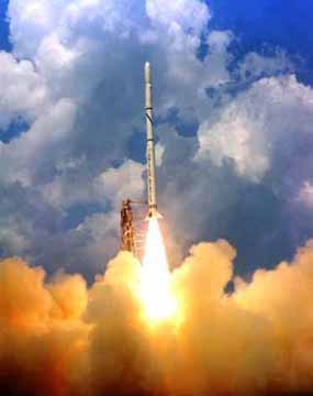
Figure 1 A rocket launched into space
Source of rocket picture: NASA Langley Research Center, Office of Education, edu.larc.nasa.gov/pstp/
If
\[m_{0} = \text{initial mass of rocket at}\ t = 0\ \text{(kg)},\]
\[q = \text{rate at which fuel is expelled}\ \text{(kg/s)},\]
\[u = \text{velocity at which the fuel is being expelled}\ \text{(m/s)}\]
then since the fuel is expelled from the rocket, the mass of the rocket keeps decreasing with time. The mass of the rocket, \(m\) at any time, \(t\) is
\[m = m_{o} - qt \;\;\;\;\;\;\;\;\;\;\;\; (1)\]
The forces on the rocket at any time are found by applying Newton’s second law of motion. Then
\[\sum F = ma \;\;\;\;\;\;\;\;\;\;\;\; (2)\]
The upward force is due to the fuel expulsion, while the downward force is due to gravity
\[{uq} - mg = ma \;\;\;\;\;\;\;\;\;\;\;\; (3)\]
Using Equations (1) and (3) in Equation (2) gives
\[{uq} - \left( m_{o} - {qt} \right)g = \left( m_{o} - {qt} \right)a \;\;\;\;\;\;\;\;\;\;\;\; (4)\]
where
\[g = \text{acceleration due to gravity}\ \left(\text{m/s}^{2} \right)\]
From Equation (4), we get
\[a = \frac{{uq}}{m_{o} - {qt}} - g \;\;\;\;\;\;\;\;\;\;\;\; (5a)\]
\[\frac{{dv}}{dt} = \frac{{uq}}{m_{o} - {qt}} - g\;\;\;\;\;\;\;\;\;\;\;\; (5b)\]
Integrating both sides of Equation (5b) gives
\[v = - u\log_{e}( m_{0} - qt) - gt + C \;\;\;\;\;\;\;\;\;\;\;\; (6)\]
Since the rocket starts from rest
\[v = 0\ \text{at}\ t = 0\]
\[0 = - u\log_{e}(m_{o}) + C\]
\[C = u\log_{e}(m_{o})\]
Hence Equation (6) reduces to
\[v = - u\log_{e}( m_{o} - {qt}) - gt + u\log_{e}( m_{o})\]
\[\frac{{dx}}{{dt}} = u{\ lo}{g}_{e}(\frac{m_{o}}{m_{o} - {qt}}) - {gt}\;\;\;\;\;\;\;\;\;\;\;\; (7)\]
Using the following numerical values in Equation (7)
\[u = 2,000\ \text{m/s}\]
\[m_{o} = 140,000\ \text{kg}\]
\[q = 2100\ \text{kg/s}\]
\[g = 9.8\ \text{m/s}^{2}\]
\[t_{0} = 0\ \text{s}\]
\[t_{1} = 30\ \text{s}\]
gives
\[v = 2000 \log_{e}\left( \frac{14 \times 10^{4}}{14 \times 10^{4} - 2100t} \right) - 9.8t.\;\;\;\;\;\;\;\;\;\;\;\; (8)\]
Can you numerically find the acceleration at \(t = 16\ \text{s}\)? You may say that we do not need numerical or analytical differentiation to calculate the acceleration, as Equation (5a) directly gives us the acceleration of the rocket at any time. True! We are just doing this as an exercise to illustrate numerical differentiation, and we have a true expression of acceleration readily available for comparison with the numerical results.
Questions
(1) Find the acceleration of the rocket at \(t = {16} \text{ s}\).
(2) Use different numerical differentiation techniques to find the acceleration at \(t = {16} \text{ s}\). Compare these results with the exact answer.
Summary
Estimating the rate at which area of containment is spreading in a lake requires numerical differentiation.
Modeling
At about 11:56 am on June 22, 1969, near the city of Cleveland in Ohio, an oil slick on the Cuyahoga River caught fire that burned for 24 minutes. This incident on a navigable river acted as a catalyst for Congress to pass the Clean Water Act in 1972. The Federal Water Pollution Control Act prohibits the discharge of oil or oily waste substances or hazardous substances into or upon the navigable waters of the United States.
Interestingly, recreational boating is a growing activity in many waterways of the United States. Unfortunately, fuel leakages – however small – from so many boats can lead to the formation of large oil slicks. The ideal would be for the recreational boats to use fuels that can evaporate as quickly as the fuels leak onto the surface of the water.

Figure 1 Waves generated on a pond by a pebble
A new fuel for recreational boats being developed at the local university was tested at an area pond by a team of engineers. The interest is to document the environmental impact of the fuel – how quickly does the slick spread? Table 1 shows the video camera record of the radius of the wave generated by a drop of the fuel that fell into the pond. To find the rate at which the contamination spreads requires numerical differentiation.
Table 1 Radius of wave generated as a function of time.
| \(\text{Time}\ (s)\) | \(0\) | \(0.5\) | \(1.0\) | \(1.5\) | \(2.0\) | \(2.5\) | \(3.0\) | \(3.5\) | \(4.0\) | \(4.5\) | \(5.0\) |
|---|---|---|---|---|---|---|---|---|---|---|---|
| \(\text{Radius}\ (m)\) | \(0\) | \(0.236\) | \(0.667\) | \(1.225\) | \(1.886\) | \(2.635\) | \(3.464\) | \(4.365\) | \(5.333\) | \(6.364\) | \(7.454\) |
Questions
(1) Compute the rate at which the radius of the drop was changing at \(t = 2\)s and \(t = 5\)s.
(2) Estimate the rate at which the area of the contaminant was spreading across the pond at \(t=2\)s and \(t = 5\)s.
Modeling
A rectangular plate under a uniform stress, \(\sigma_{0}\), results in the stress state of
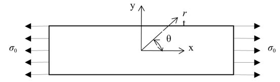
Figure 1. Rectangular plate under uniform stress.
where
\[{\sigma_{{xx}} = \sigma_{0}}\]
\[{\sigma_{{yy}} = 0}\]
\[{\sigma_{{zz}} = 0}\]
If the plate now has changed in the cross-section, the normal stresses will increase as a result of these changes. For example, if there is a circular hole in the plate (Figure 2) and it is subjected to the same uniform stress, \(\sigma_{0}\), then stresses in the plate would increase. For example, if the radius of the hole in the plate was small compared to the length and width of the plate, the solution can be found analytically for \(\sigma_{{xx}} = 3\sigma_{0}\) at \(r = a\), \(\displaystyle \theta = \pm \frac{\pi}{2}\).
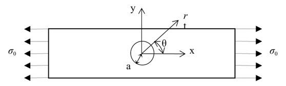
Figure 2. Rectangular plate with circular hole of radius a under uniform stress.
This in fact is the highest normal stress that occurs in such a case. To specify such stresses we define a term called stress concentration, k, that is
\[k = \frac{{Maximum\ Stress}}{{Nominal\ Stress}}\]
So in this case
\[\begin{split} k &=\frac{(3\sigma _0)}{\sigma _0}\\ &= 3\end{split}\]
Now what happens when the radius of the hole is not small as compared to the length and width of the plate? In most cases, the stresses cannot be found analytically, and we need to solve the problem using numerical techniques. One such method is called the finite difference method. Here is how it works for this problem. The partial differential equations for the plane stress problem are given by
\[\frac{\partial^{2}u}{\partial x^{2}} + \frac{\left( 1 - \upsilon \right)}{2}\frac{\partial^{2}v}{\partial y^{2}} + \frac{\left( 1 + \upsilon \right)}{2}\frac{\partial^{2}v}{\partial x\partial y} = 0\;\;\;\;\;\;\;\;\;\;\;\; (1)\]
\[\frac{\partial^{2}v}{\partial y^{2}} + \frac{\left( 1 - \upsilon \right)}{2}\frac{\partial^{2}u}{\partial x^{2}} + \frac{\left( 1 + \upsilon \right)}{2}\frac{\partial^{2}u}{\partial x\partial y} = 0\;\;\;\;\;\;\;\;\;\;\;\; (2)\]
Where
\[u = \text{displacement in x-direction}\]
\[v = \text{displacement in y-direction}\]
\[\upsilon = \text{Poisson's ratio}\]
To apply the finite difference method, the rectangular plate with the hole would be divided into \((m-1)\) segments along the x-axis and \((n-1)\) segments along the y-axis as shown in Figure 3. This results in nodes in the plate.
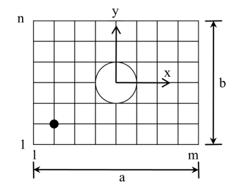
Figure 3 Finite Difference Nodes of Rectangular Plate with Hole.
Now at each node such as a general node (i,j) where the surrounding nodes do not have a node on the hole, the forward divided difference approximations can be applied as
\[\frac{\partial^{2}u}{\partial x^{2}}\left| i,j \right.\ \approx \frac{u_{i + 1,j} - 2u_{i,j} + u_{i - 1,j}}{\left( \Delta x \right)^{2}}\ \ \ (3)\]
\[\frac{\partial^{2}v}{\partial y^{2}}\left| i,j \right.\ \approx \frac{v_{i,j + 1} - 2v_{i,j} + v_{i,j - 1}}{\left( \Delta y \right)^{2}}\ \ \ (4)\]
\[\frac{\partial^{2}v}{\partial x\partial y}\left| i,j \right.\ \approx \frac{v_{i + 1,j + 1} - v_{i + 1,j - 1} - v_{i - 1,j + 1} - v_{i - 1,j - 1}}{\left( \Delta x \right)\left( \Delta y \right)}\ \ \ (5)\]
\[\frac{\partial^{2}u}{\partial x\partial y}\left| i,j \right.\ \approx \frac{u_{i + 1,j + 1} - u_{i + 1,j - 1} - u_{i - 1,j + 1} - u_{i - 1,j - 1}}{\left( \Delta x \right)\left( \Delta y \right)}\ \ \ (6)\]
Substituting these approximations (equations 3-6) in equation (1) and (2) gives
\[\begin{split} &\frac{u_{i + 1,j} - 2u_{i,j} + u_{i - 1,j}}{\left( \Delta x \right)^{2}} + \frac{\left( 1 - \upsilon \right)}{2}\left\lbrack \frac{v_{i,j + 1} - 2v_{i,j} + v_{i,j - 1}}{\left( \Delta y \right)^{2}} \right\rbrack\\ &+ \frac{\left( 1 + \upsilon \right)}{2}\left\lbrack \frac{v_{i + 1,j + 1} - v_{i + 1,j - 1} - v_{i - 1,j + 1} - v_{i - 1,j - 1}}{\left( \Delta x \right)\left( \Delta y \right)} \right\rbrack = 0\end{split} \;\;\;\;\;\;\;\;\;\;\;\; (7)\]
\[\begin{split} &\frac{v_{i,j + 1} - 2v_{i,j} + v_{i,j - 1}}{\left( \Delta y \right)^{2}} + \frac{\left( 1 - \upsilon \right)}{2}\left\lbrack \frac{u_{i + 1,j} - 2u_{i,j} + u_{i - 1,j}}{\left( \Delta x \right)^{2}} \right\rbrack\\ &+ \frac{\left( 1 + \upsilon \right)}{2}\left\lbrack \frac{u_{i + 1,j + 1} - u_{i + 1,j - 1} - u_{i - 1,j + 1} - u_{i - 1,j - 1}}{\left( \Delta x \right)\left( \Delta y \right)} \right\rbrack = 0\end{split} \;\;\;\;\;\;\;\;\;\;\;\; (8)\]
Similarly one would write equations for the nodes that are around the hole and also for ones that are surrounded by the nodes on the hole. This is out of the scope of this topic but needs to be appreciated. We will also skip the application of boundary conditions at the outer four edges of the plate as well as the radius of the hole. However, one needs to realize that once all the equations are defined, we get as many unknowns (6: the displacement in the x- and y-directions, at each node) as we have equations by the approximations to equations (1) and (2), as well as the boundary conditions. This results in solving simultaneous linear equations. After the displacements are calculated, one can find stress and strain in the plate to consequently find the stress concentration. As an example, the problem description of one such case is given below.
To find the stresses and hence the stress concentration factor, one needs to find the derivatives of these displacements. In Table 1 the radial displacements \(u\) are given along the \(y\) -axis. The radius of the hole is 1.0 cm.
a) At \(x = 0\), if the radial strain \(\varepsilon_{r}\) is given by \(\displaystyle\varepsilon_{r} = \frac{\partial u}{\partial r}\), find the radial strain at \(r = 1.1{cm}\) using the forward divided difference method.
b) If the tangential strain at \(r = 1.1{cm},\ \theta = 90{^\circ}\) is given to you as \(\varepsilon_{\theta} = 0.0029733\), find the hoop stress, \(\sigma_{\theta}\), at \(r = 1.1{\ cm},\ \theta = 90{^\circ}\) if \(\displaystyle \sigma_{\theta} = \frac{E}{1 - \nu^{2}}(\varepsilon_{r} + \nu\varepsilon_{\theta})\), where \(E = 200 \text{ GPa and}\ \nu\ = 0.3\).
Table 1 Radial displacement as a function of location.
| \(r\;({cm})\) | \(u\;({cm})\) |
|---|---|
| \(1.0\) | \(–0.0010000\) |
| \(1.1\) | \(–0.0010689\) |
| \(1.2\) | \(–0.0011088\) |
| \(1.3\) | \(–0.0011326\) |
| \(1.4\) | \(–0.0011474\) |
| \(1.5\) | \(–0.0011574\) |
| \(1.6\) | \(–0.0011650\) |
| \(1.7\) | \(–0.0011718\) |
| \(1.8\) | \(–0.0011785\) |
| \(1.9\) | \(–0.0011857\) |
Modeling
Human vision is an intriguing ability. The fact that we can effortlessly recognize objects, people, and read this document belies the complexity of the task that a significant portion of our brain is devoted to solving. You might be surprised to learn that this almost photographic perception of the world that we have is not what our eyes send to our brain. What we perceive is a reconstruction from the noisy, shaky output of elementary “things” or “features” detected in the retina. There is strong evidence that the first level of processing done in the retina involves detecting something called “edges” or positions of transitions from dark to bright or bright to dark points in the images. These points usually coincide with boundaries of things.
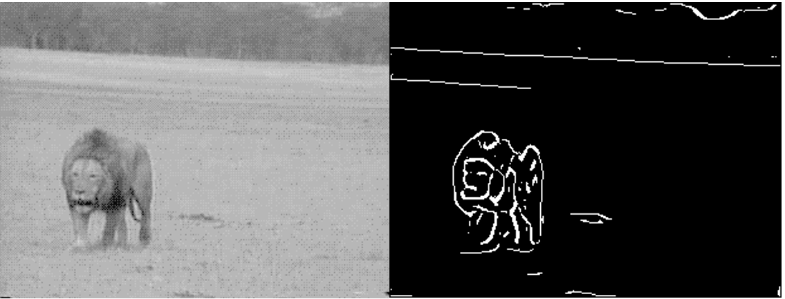
Figure 1 On left is an image, with the corresponding edge image shown on the right.
In Figure 1 above we see an example of an edge image. This process of “detecting” edges in an image is called edge detection and can be modeled as a differentiation process. In this module we will look into this differentiation process.
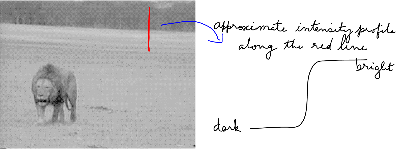
Figure 2 Edges corresponds to points in the image where there are intensity changes.
In the above Figure we see the profile of the intensity value along a line (shown in red) cutting an edge in the image. We represent small values to represent dark points in the image and large values to detect bright regions in the image. The value increases and saturates to the value of the bright region. The edges can be marked at point of the maximum change in intensity, or where the derivative is a maximum. We will study the behavior of this derivative for a class of models of the edges.
Example
One way to model the edge, which is denote by \(e^{x}\), where \(x\) is the direction perpendicular to the edge, is using exponential functions.
\[e(x) = \left\{ \begin{matrix} 1 - e^{( - ax)}\begin{matrix} \ & \forall x \geq 0 \\ \end{matrix} \\ e^{(ax)} - 1\begin{matrix} \ & \forall x \leq 0 \\ \end{matrix} \\ \end{matrix} \right.\ \;\;\;\;\;\;\;\;\;\;\;\; (1)\]
Plots of this function for various values of \(a\) are shown in the Figure 3 below. Ignore the fact that we have used negative values to represent intensity. We can always add a constant to shift the function “up”, but the constant will not have any impact on the final derivative.
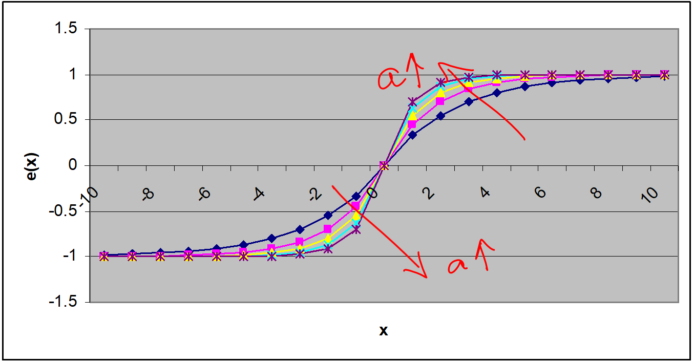
Figure 3 Plot of the exponential edge profile model for various values of the modeling parameter \(a\).
The derivative of this profile model is given by
\[e(x) = \left\{ \begin{matrix} 1 - e^{( - ax)}\begin{matrix} \ & \forall x \geq 0 \\ \end{matrix} \\ e^{(ax)} - 1\begin{matrix} \ & \forall x \leq 0 \\ \end{matrix} \\ \end{matrix} \right.\ \;\;\;\;\;\;\;\;\;\;\;\; (2)\]
(Note that at \(x = 0\) both the derivatives have the same value of \(a\); this shows that the function we used to model the edge profile is continuous in value and first derivative. This is just an aside fact that you might store in your brain for future use!)
What happens to the derivative as the underlying edge gets sharper? We see from Figure 4 that the value of the derivative gets larger and the peak gets sharper. Thus, strong edges, that is, edges with sharp intensity transitions will results in stronger response.
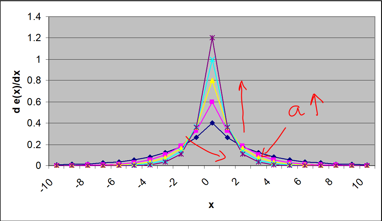
Figure 4 Plot of the derivative of the edge profile as the parameter \(a\) is increased.
Questions
(1) What kind of “edge” is represented by the following edge profile model?
\[e(x) = e^{( - ax^{2})}\]
Answer: Line edge: the edge will appear as a white line in a dark background. What happens to the width of this line as you change \(a\).
(2) Compute the first derivative of the above function given in #1.
(3) Where, that is for what values of \(x\), does this derivative reach a maximum or a minimum values? What happens to the distance between the maximum and minimum value locations as \(a\) is increased?
(4) Where is the value of the derivative zero?
Modeling
The vast majority of commercial and industrial loads are inductive in character. Many electrical consumers find it advantageous to use capacitor banks to adjust their power factor toward 1.0 to avoid extensive rate penalties from their power utility. As load conditions change, it becomes necessary to add or remove capacitors from the bank. The most opportune time to do this is when the voltage across the capacitor is zero to avoid arcing and damages to the switches. Since the switches are slower than the AC waveforms, it is necessary to use a derivative of the voltage to anticipate the zero crossing.
Electrical systems are used for a wide-array of applications in the commercial and industrial world. Many of them perform physical work using motors, compressors, solenoids, and similar components. In almost all cases, these devices employ electro-magnetic principles and are thus inductive in nature. This presents an electrical load that result in a power factor lagging. Whenever the power factor of a load is not 1.0 (leading or lagging), it results in a discrepancy between the apparent power delivered to the load and the real power consumed by the load.
For most commercial and industrial power consumers, as opposed to residential, the electrical power utility bases its rate charge on the apparent power delivered. This often takes the form of a significant penalty for power factors much below 1.0 (e.g. 0.8). To help correct the power factor it is common to add capacitor banks in parallel with a load that can shift a lagging power factor toward 1.0. Under ideal circumstances, the capacitors could be connected and disconnected from the circuit at any time. Under practical conditions, however, this is not advisable.
The amount of energy in a capacitor is directly related to the voltage across the capacitor as shown in the familiar equation
\[E_{c} = \frac{1}{2}CV_{c}^{2} \;\;\;\;\;\;\;\;\;\;\;\; (1)\]
When a switch tries to disconnect the capacitor, the energy resists this disconnection, and the result is often sparking and gapping as the switch opens. This not only is a significant source of noise in the circuit, but it also results in damage to the switch that greatly reduces its effective service life. The solution to this problem is quite simple; just open the switch when the stored energy is zero. This, of course, occurs when the voltage across the capacitor is zero.
Unfortunately, it is not just a matter of monitoring the voltage and activating the switch when the voltage is zero. The normal frequency for AC power systems is 60 Hz (50 Hz in Europe). This means that there are 120 zero crossings per second and the typical mechanical switch is simply not fast enough to react “instantaneously” at the zero crossing. To deal with this a smart capacitor bank switch is needed. It monitors the voltage and using numerical methods anticipates the point of zero crossing and initiates the switch action enough in advance to have it occur as close to the zero crossing as possible.
This can be done using a first-order approximation of the Taylor Series as shown by the following equations as well as Figure 1.
\[f\left( t + \Delta t \right) \cong f\left( t \right) + f^{'}\left( t \right)\Delta t = 0 \;\;\;\;\;\;\;\;\;\;\;\; (2)\]
\[\Delta t \cong - \frac{f\left( t \right)}{f^{'}\left( t \right)} \;\;\;\;\;\;\;\;\;\;\;\; (3)\]
If this formula looks a bit familiar, it is the same one used as the basis for Newton’s Method as it is commonly used in root finding algorithms.
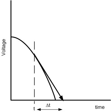
Figure 1 Illustration of Zero-Crossing Prediction Using First-Order Taylor Series
Suppose a system containing a capacitor bank has been constructed and the data of Table 1 was sampled during operation. Using a numerical differentiating algorithm determine the derivative at each point and use the Taylor Series approximation to determine the value of \(\Delta t\) which gives the future estimate of the zero crossing. Keep in mind that when \(\Delta t\) is determined to be negative then the voltage has already crossed the zero point and it will be necessary to wait for the next half cycle of the waveform.
Most numerical methods for taking a derivative (e.g. the Central Difference Method) rely on samples taken both before and after the period in question. In this problem that is not practical since our desire it to anticipate the future zero crossing at which the power should be turned off. Repeat your prior analysis using a differentiation algorithm that is one-sided, that is, one that only uses prior samples to determine the present value of the voltage’s derivative.
Table 1 Voltage Samples
| Time | Voltage | Time | Voltage |
|---|---|---|---|
| \(1\) | \(0.62161\) | \(13\) | \(-0.210796\) |
| \(2\) | \(0.362358\) | \(14\) | \(0.087499\) |
| \(3\) | \(0.070737\) | \(15\) | \(0.377978\) |
| \(4\) | \(-0.227202\) | \(16\) | \(0.634693\) |
| \(5\) | \(-0.504846\) | \(17\) | \(0.834713\) |
| \(6\) | \(-0.737394\) | \(18\) | \(0.96017\) |
| \(7\) | \(-0.904072\) | \(19\) | \(0.999859\) |
| \(8\) | \(-0.989992\) | \(20\) | \(0.950233\) |
| \(9\) | \(-0.98748\) | \(21\) | \(0.815725\) |
| \(10\) | \(-0.896758\) | \(22\) | \(0.608351\) |
| \(11\) | \(-0.725932\) | \(23\) | \(0.346635\) |
| \(12\) | \(-0.490261\) | \(24\) | \(0.053955\) |
Questions
(1) What effect does the order of your differentiation algorithm have on the ability to predict correctly the point of zero crossing? Is there an order at which there are diminishing returns on the ability to identify the point of zero crossing?
(2) Using a higher-order approximation to the Taylor Series will also improve the prediction of the zero crossing, especially when it is a bit distant. Use a second-order model of the Taylor Series that requires both the first- and second-order derivative to determine \(\Delta t\).
(3) In a real AC system, there could easily be quite a large amount of noise on the sampled voltages. Are there any reasonable algorithms for minimizing the effects this noise has on the results?
(4) The typical AC system in the United States uses a 60 Hz frequency (50 Hz in Europe). What is a reasonable sampling rate to use for the voltage sensor? How much does the required length for \(\Delta t\) impact your answer. Did you account for the problem of question (c) in your answer?
(5) As in the data of Table 1, the samples have not been synchronized well with the cycles of the AC waveform (that is why you do not see 1 or -1 among the samples). Can you suggest a mechanism for bringing the samples in better synchronization with the cycles?
(6) Most industrial smart-sensors for this application use a prediction and correction method to detect the zero crossing, that is, they predict the crossing and then see how close they are for a few cycles prior to the actual disconnecting action. How might such an algorithm be structured?
(7) Would there be any advantage in using an interpolation or curve fitting algorithm (e.g. regression to a sinusoid) to better select the instant of true zero voltage?
(8) In a system with multiple loads (e.g. a three-phase system), the best instant of shut off for one phase of the capacitor banks may not be the best for the others. Is there any way to determine the point of best compromise or is it simply better to shut each of them off at the zero crossing and tolerate the temporary imbalance to the three-phase system?
Modeling
The following is from a Firestone recall page (www.firestone-tire-recall.com/pages/overview.html -dead link).
“The Firestone tire recall is perhaps the most deadly auto safety crisis in American history. US regulators on 16 October, 2000 have raised the death count to 119 (the death count has steadily risen from 62, later to 88 and 101 deaths reported on 9/20/2000). Experts believe there may be as many as 250 deaths and more than 3000 catastrophic injuries associated with the defective tires. Most of the deaths occur in accidents involving the Ford Explorer which tends to rollover when one of the tires blows out.
In May 2000, the National Highway Transportation Safety Administration issued a letter to Ford and Firestone requesting information about the high incidence of tire failure on Ford Explorer vehicles. During July, Ford obtained and analyzed the data on tire failure. The data revealed that \(15^{\prime\prime}\) ATX and ATX II models and Wilderness AT tires had very high failure rates: the tread peels off. Many of the tires were made at a Decatur, Illinois plant. When the tires fail, the vehicle often rolls over and kills the occupants.
Ford Officials estimate the defect rate is 241 tires per million for 15 inch ATX and ATX II tires. By contrast Ford says there are no defects in 16 inch tires per million and only 2.3 incidents per million on other tires.
On August 9th, both companies decided on the recall. Ford and Firestone disagreed as to how to break the news. Bridgestone/Firestone officials wanted to read a statement at a joint briefing without answering any questions. Ford strongly disagreed with this strategy and warned of disaster if they refused questions. Ultimately questions were asked, many of them remain unanswered.”
In our daily lives, we depend on a lot of different products. Their inability to perform may cause us inconveniences and sometimes more dire consequences as in the Firestone tire recall case. Therefore, companies are required to carefully study, document and control the reliability of their products before they are released to the market.
Reliability Function
Reliability function is frequently used to describe the probability of an item operating under certain conditions for a certain amount of time without failure. The reliability function is a function of time, in that every reliability value has an associated time value. In other words, one must specify a time value with the desired reliability value, that is, 95% reliability at 100 hours.
Mathematically, the reliability function \(R(t)\) is the probability that a system will be successfully operating without failure in the interval from \(t = 0\) to \(t\),
\[\begin{split} R(t) &= P(T > t),t \geq 0\\ &= \int_{t}^{\infty}{f(s)ds} \end{split} \;\;\;\;\;\;\;\;\;\;\;\; (1)\]
where \(T\) is a random variable representing the failure time or time-to-failure and \(f(t)\) is the time to failure distribution function. More often than not, the time to failure distribution function is denoted by exponential, Weibull, normal or lognormal distribution based on the characteristics of the underlying product or the system. However, for complex practical systems the above distributions may not provide an accurate fit for the time to failure distribution function.
Also of interest is the failure distribution function \(F(t)\) which describes the probability of an item failing before a certain period of time. As you may guess, the failure distribution function and the reliability function are related to each other by
\[F(t) + R(t) = 1 \;\;\;\;\;\;\;\;\;\;\;\; (2)\]
where
\[F(t) = \int_{0, - \infty}^{t}{f(s)ds} \;\;\;\;\;\;\;\;\;\;\;\; (3)\]
Failure Rate Function
The failure rate function, or hazard function, is also very important in reliability analysis because it specifies the rate of the system aging. The failure rate function \(h(t)\) is defined as:
\[\begin{split} h\left(t\right)&=\lim_{{\Delta\ t}\rightarrow0}\frac{R\left(t\right)-R\left(t+{\Delta\ t}\right)}{{\Delta\ tR}\left(t\right)}\\ &= \frac{f(t)}{R(t)}\end{split} \;\;\;\;\;\;\;\;\;\;\;\; (4)\]
The importance of the failure rate function is that it indicates the changing rate in the aging behavior over the life of a population of components. For example, if the time to failure distribution function follows an exponential distribution with parameter \(\lambda\), then the failure rate function is
\[\begin{split} h(t)&=\frac{f(t)}{R(t)}\\ &= \frac{\lambda e^{-{\lambda t}}}{e^{-{\lambda t}}} \\ &= \lambda \end{split} \;\;\;\;\;\;\;\;\;\;\;\; (5)\]
This means that the failure rate function of the exponential distribution is a constant. In this case, the system does not have any aging property. This assumption is usually valid for software systems. However, for hardware systems, the failure rate could have other shapes. More information regarding reliability analysis can be found in [1].
A series systems, shown in Figure 1, is defined as \(n\) independent components arranged in series. The reliability of the system at time \(t\),\(R_{s}(t)\), is the probability that all components survive to time \(t\), or in other words,
\[R_{s}(t) = R_{1}(t)R_{2}(t)\ldots R_{n}(t) = \prod_{i = 1}^{n}{R_{i}(t)} \;\;\;\;\;\;\;\;\;\;\;\; (6)\]
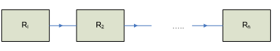
Figure 1 Block diagram of a series system
The following example relies on the research published in [2]. Low power portable direct methanol fuel cell (DMFC) systems provide higher energy density and longer operational life compared with Li-ion batteries widely used in portable electronic devices such as cellular phones, laptops, etc.
DMFC systems consist of three main subsystems, namely the fuel cell stack, fuel tank and the Balance of Plant which are assumed to be independently connected to each other in series as shown in Figure 2. These systems are still an immature technology and there is no publicly available reliable failure data for DMFC components.
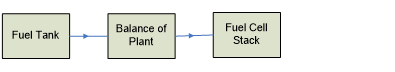
Figure 2 Block diagram of a DFMC system
Consider the following reliability data in Table 1 for the DMFC system.
Table 1. Reliability of DFMC system
| \(t\ (hrs)\) | \(0\) | \(1\) | \(10\) | \(100\) | \(1000\) | \(2000\) | \(3000\) | \(4000\) | \(5000\) |
|---|---|---|---|---|---|---|---|---|---|
| \(R(t)\) | \(1\) | \(0.9999\) | \(0.9998\) | \(0.9980\) | \(0.9802\) | \(0.9609\) | \(0.9419\) | \(0.9233\) | \(0.9050\) |
Questions
(1) Calculate the value of the failure rate function, \(h(t)\) at \(t = 10\) hours.
(2) Calculate the value of the failure rate function, \(h(t)\) at \(t = 2000\) hours.
(3) Calculate the value of the failure rate function, \(h(t)\) at \(t = 4000\) hours.
(4) Compare the results you have in questions 1-3. What can be said about the failure rate function and the time to failure distribution function \(F(t)\) of the DMFC system based on the data provided?
(5) You are told that the estimated failure rate for the fuel tank and the fuel cell stack are constant with values \(5.42 \times 10^{- 8}\) and \(7.78 \times 10^{- 6}\). Can you calculate an estimate the failure rate for the Balance of Plant?
(6) If you are told that the time to failure distribution function of the DFMC system is exponential with parameter \(\lambda = 1.21 \times 10^{- 5}\), calculate the accuracy of your answers to questions 1-3.
References
[1] E. A. Elsayed (1996), Reliability Engineering, Addison-Wesley.
[2] N.S. Sisworahardjo, M.S.Alam and G. Aydinli, “Reliability and availability of low power portable direct methanol fuel cells”, Journal of Power Sources, 177, 2008, p.412-418.
[3] Firestone and Ford tire controversy, Wikipedia page, https://en.wikipedia.org/wiki/Firestone_and_Ford_tire_controversy, last accessed May 26, 2021.
Summary
Finding how the coefficient of linear thermal expansion varies with temperature requires numerical differentiation.
Modeling
To make the fulcrum (Figure 1) of a bascule bridge, a long hollow steel shaft called the trunnion is shrink fit into a steel hub.
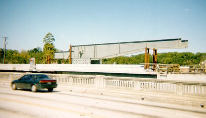
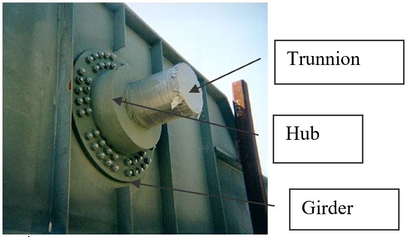
Figure 1 Trunnion-Hub-Girder (THG) assembly.
This is done by first immersing the trunnion in a cold medium such as a dry-ice/alcohol mixture. After the trunnion reaches a steady-state temperature, that is the temperature of the cold medium, the trunnion outer diameter contracts, is taken out and slid through the hole of the hub (Figure 2).
When the trunnion heats up, it expands and creates an interference fit with the hub. In 1995, on one of the bridges in Florida, this assembly procedure did not work as designed. Before the trunnion could be inserted fully into the hub, the trunnion got stuck. So a new trunnion and hub had to be ordered worth $50,000. Coupled with construction delays, the total loss ran into more than a hundred thousand dollars.
Why did the trunnion get stuck - because the trunnion had not contracted enough to slide through the hole.
Now the same designer is working on making the fulcrum for another bascule bridge. Can you help him so that he does not make the same mistake?
For this new bridge, he needs to fit a hollow trunnion of outside diameter \(12.363^{\prime\prime}\) in a hub of inner diameter \(12.358^{\prime\prime}\). His plan is to put the trunnion in dry-ice/alcohol mixture (temperature of dry-ice/alcohol mixture is \(- 108{^\circ}F\)) to contract the trunnion so that it can be slid through the hole of the hub. To slide the trunnion without sticking, he has also specified a diametric clearance of at least \(0.01^{\prime\prime}\). Assume the room temperature is \(80{^\circ}F\), is immersing it in a dry-ice/alcohol mixture a correct decision?
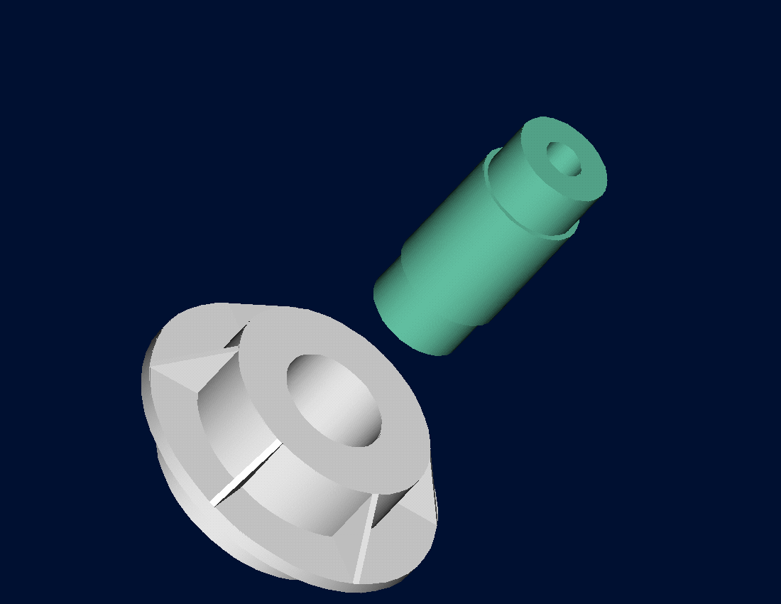
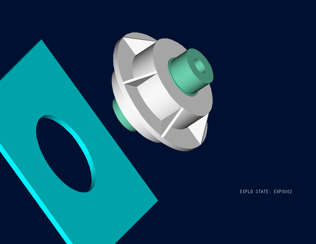
Figure 2 Trunnion slid through the hub after contracting
Looking at the records of the designer for the previous bridge where the trunnion got stuck in the hub, it was found that he used the thermal expansion coefficient at room temperature to calculate the contraction in the trunnion diameter. In that case, the reduction, \(\Delta D\) in the outer diameter of the trunnion is
\[\Delta D = D\alpha\Delta T\;\;\;\;\;\;\;\;\;\;\;\; (1)\]
where
\[D = \text{outer diameter of the trunnion,}\]
\[\alpha =\text{coefficient of thermal expansion coefficient at room temperature,}\]
\[\Delta T =\text{change in temperature,}\]
Given
\[D = 12.363^{\prime\prime}\]
\[\alpha = 6.817 \times 10^{- 6}\frac{{in}}{{in/}{^\circ}F}\ \text{at}\ 80{^\circ}F\]
\[\begin{split} \Delta T &= T_{{fluid}} - T_{{room}}\\ &= - 108 - 80\\ &= - 188{^\circ}F \end{split}\]
where
\[T_{{fluid}} =\text{temperature of dry-ice/alcohol mixture}\]
\[T_{{room}} =\text{room temperature}\]
The reduction in the trunnion outer diameter from Equation (1) is given by
\[\begin{split} \Delta D &= 12.363 \times \left( 6.47 \times 10^{- 6} \right)\left( - 188 \right)\\ &=- 0.01504^{\prime\prime} \end{split}\]
So the trunnion is predicted to reduce in diameter by \(0.01504^{\prime\prime}\). But is this enough reduction in diameter? As per the specifications, he needs the trunnion to contract by
\[\begin{split} &= \text{trunnion outside diameter} - \text{hub inner diameter} + \text{diametral clearance}\\ &= 12.363^{\prime\prime} - 12.358^{\prime\prime} + 0.01^{\prime\prime}\\ &= 0.015^{\prime\prime} \end{split}\]
So, according to his calculations, it is enough to put the steel trunnion in dry-ice/alcohol mixture to get the desired contraction of \(0.015^{\prime\prime}\) as he is predicting a contraction of \(0.01504^{\prime\prime}\).
But as shown in Figure 3, the coefficient of linear thermal expansion of steel decreases with a decrease in temperature and is not constant over the range of temperature the trunnion goes through. Hence the above formula (Equation 1) would overestimate the thermal contraction. This assumption is the mistake he made in the calculations for the earlier bridge.
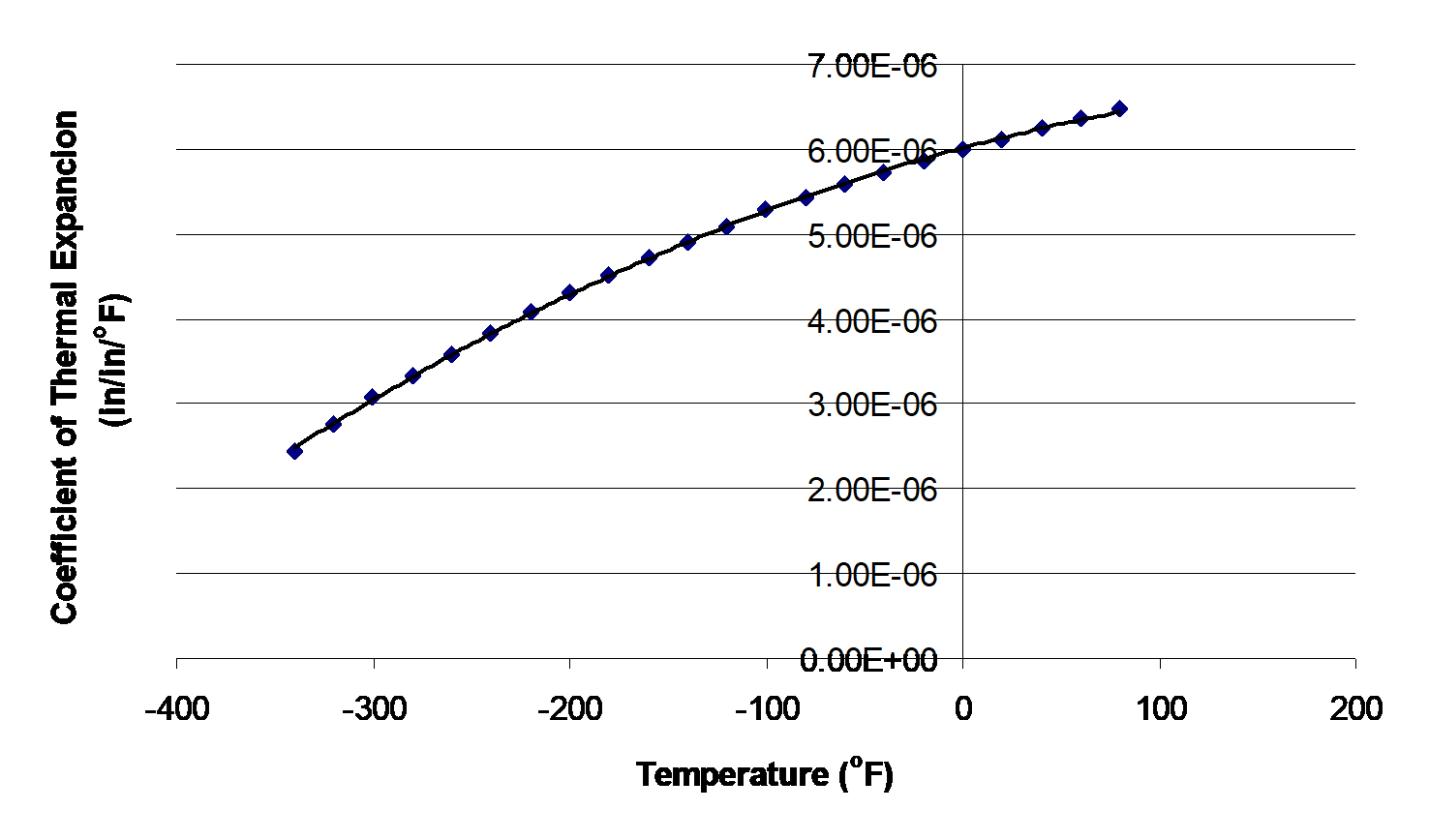
Figure 3 Varying coefficient of linear thermal expansion as a function of temperature for cast steel.
To find the contraction of a steel cylinder immersed in a bath of liquid nitrogen, one needs to know the coefficient of linear thermal expansion data as a function of temperature. This data is given for steel in Table 1.
Table 1 Coefficient of linear thermal expansion as a function of temperature
| Temperature, T (\({^\circ}F\)) | Coefficient of linear thermal expansion, \(\alpha\) (\({\mu{in}/}{{in/}{^\circ}F}\)) |
|---|---|
| \(80\) | \(6.47\) |
| \(40\) | \(6.24\) |
| \(-40\) | \(5.72\) |
| \(-120\) | \(5.09\) |
| \(-200\) | \(4.30\) |
| \(-280\) | \(3.33\) |
| \(-340\) | \(2.45\) |
An exercise to appreciate the way the thermal expansion coefficient changes with respect to the temperature is to look at the slope of the thermal expansion coefficient with respect to temperature at low and high temperatures.
Questions
(1) Using the data from Table 1, is the rate of change of coefficient of thermal expansion with temperature more at \(T = 80{^\circ}F\) than at \(T = - 340{^\circ}F\) ? Use any numerical differentiation technique.
(2) The data given in Table 1 can be regressed to \(\alpha = a_{0} + a_{1}T + a_{2}T^{2}\) to get \(\alpha = {6.0217} \times {1}{0}^{- 6} + {6.2782} \times {1}{0}^{- 9}T - {1.2218} \times {1}{0}^{- {11}}T^{2}\). Compare the results from Problem 1 if you use the regression curve to find the rate of change of coefficient of thermal expansion with respect to temperature at \(T = 80{^\circ}F\) and at \(T = - 340{^\circ}F\).