Chapter 05.03: Newton’s Divided Difference Method of Interpolation
Learning Objectives
After successful completion of this lesson, you should be able to:
1) find the interpolant through the Newton’s divided difference interpolation,
2) choose the correct data points for interpolation,
3) solve problems using the Newton’s divided difference interpolation,
4) use Newton’s divided difference interpolants to find derivatives of discrete functions,
5) use the Newton’s divided difference interpolants to find integrals of discrete functions.
Introduction
Polynomial interpolation involves finding a polynomial of order \(n\) that passes through the \(n + 1\) points. One of the methods of interpolation is called Newton’s divided difference polynomial method. Other methods include the direct method and the Lagrangian interpolation method. We will discuss Newton’s divided difference polynomial method in this chapter.
Newton’s Divided Difference Polynomial Method
To illustrate this method, linear and quadratic interpolation is presented first. Then, the general form of Newton’s divided difference polynomial method is presented. To illustrate the general form, cubic interpolation is shown in Figure 1.
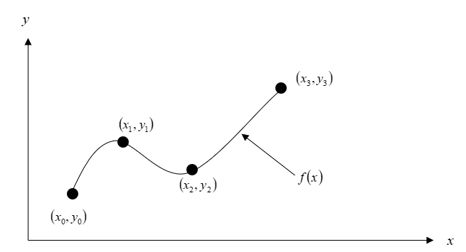
Figure 1 Interpolation of discrete data.
Linear Interpolation
Given \((x_{0},y_{0})\) and \((x_{1},y_{1}),\) fit a linear interpolant through the data. Noting \(y = f(x)\) and \(y_{1} = f(x_{1})\), assume the linear interpolant \(f_{1}(x)\) is given by (Figure 2)
\[f_{1}(x) = b_{0} + b_{1}(x - x_{0})\]
Since at \(x = x_{0}\),
\[f_{1}(x_{0}) = f(x_{0}) = b_{0} + b_{1}(x_{0} - x_{0}) = b_{0}\]
and at \(x = x_{1}\),
\[\begin{split} f_{1}(x_{1}) &= f(x_{1}) = b_{0} + b_{1}(x_{1} - x_{0})\\ &= f(x_{0}) + b_{1}(x_{1} - x_{0}) \end{split}\]
giving
\[b_{1}=\frac{f\left(x_{1}\right)-f\left(x_{0}\right)}{x_{1}-x_{0}}\]
So
\[b_{0} = f(x_{0})\] \[b_{1}=\frac{f\left(x_{1}\right)-f\left(x_{0}\right)}{x_{1}-x_{0}}\]
giving the linear interpolant as
\[f_{1}(x) = b_{0} + b_{1}(x - x_{0})\]
\[f_{1}(x) = f(x_{0}) + \frac{f(x_{1}) - f(x_{0})}{x_{1} - x_{0}}(x - x_{0})\]
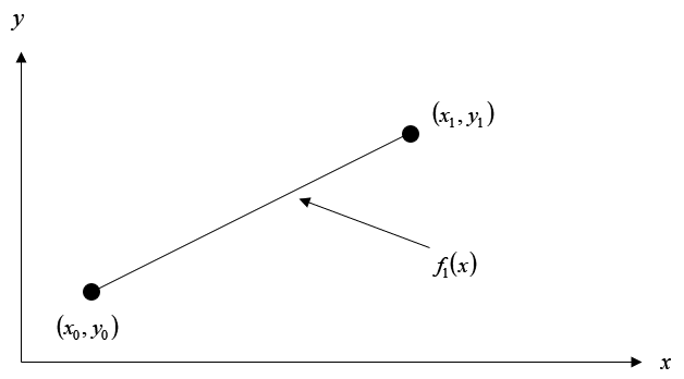
Figure 2 Linear interpolation.
Example 1
The upward velocity of a rocket is given as a function of time in Table 1 (Figure 3).
Table 1 Velocity as a function of time.
| \(t\ (s)\) | \(v(t)\ (\text{m/s})\) |
|---|---|
| \(0\) | \(0\) |
| \(10\) | \(227.04\) |
| \(15\) | \(362.78\) |
| \(20\) | \(517.35\) |
| \(22.5\) | \(602.97\) |
| \(30\) | \(901.67\) |
Determine the value of the velocity at \(t = 16\) seconds using first order polynomial interpolation by Newton’s divided difference polynomial method.
Solution
For linear interpolation, the velocity is given by
\[v(t) = b_{0} + b_{1}(t - t_{0})\]
Since we want to find the velocity at \(t = 16\), and we are using a first order polynomial, we need to choose the two data points that are closest to \(t = 16\) that also bracket \(t = 16\) to evaluate it. The two points are \(t = 15\) and \(t = 20\).
Then
\[t_{0} = 15,\ v(t_{0}) = 362.78\]
\[t_{1} = 20,\ v(t_{1}) = 517.35\]
gives
\[\begin{split} b_{0} &= v(t_{0})\\ &= 362.78\\ \end{split}\]
\[\begin{split} b_{1} &= \frac{v(t_{1}) - v(t_{0})}{t_{1} - t_{0}}\\ &= \frac{517.35 - 362.78}{20 - 15}\\ &= 30.914 \end{split}\]
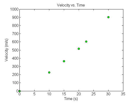
Figure 3 Graph of velocity vs. time data for the rocket example.
Hence
\[\begin{split} v(t) &= b_{0} + b_{1}(t - t_{0})\\ &= 362.78 + 30.914(t - 15),\ 15 \leq t \leq 20 \end{split}\]
At \(t = 16,\)
\[\begin{split} v(16) &= 362.78 + 30.914(16 - 15)\\ &= 393.69\text{ m/s} \end{split}\]
If we expand
\[v(t) = 362.78 + 30.914(t - 15),\ 15 \leq t \leq 20\]
we get
\[v(t) = - 100.93 + 30.914t,\ 15 \leq t \leq 20\]
and this is the same expression as obtained in the direct method.
Quadratic Interpolation
Given \((x_{0},y_{0}),\) \((x_{1},y_{1}),\) and \((x_{2},y_{2}),\) fit a quadratic interpolant through the data. Noting \(y = f(x),\) \(y_{0} = f(x_{0}),\) \(y_{1} = f(x_{1}),\) and \(y_{2} = f(x_{2}),\) assume the quadratic interpolant \(f_{2}(x)\) is given by
\[f_{2}(x) = b_{0} + b_{1}(x - x_{0}) + b_{2}(x - x_{0})(x - x_{1})\]
At \(x = x_{0}\),
\[\begin{split} f_{2}(x_{0}) &= f(x_{0}) = b_{0} + b_{1}(x_{0} - x_{0}) + b_{2}(x_{0} - x_{0})(x_{0} - x_{1})\\ &= b_{0} \end{split}\]
\[b_{0} = f(x_{0})\]
At \(x = x_{1}\)
\[f_{2}(x_{1}) = f(x_{1}) = b_{0} + b_{1}(x_{1} - x_{0}) + b_{2}(x_{1} - x_{0})(x_{1} - x_{1})\]
\[f(x_{1}) = f(x_{0}) + b_{1}(x_{1} - x_{0})\]
giving
\[b_{1} = \frac{f(x_{1}) - f(x_{0})}{x_{1} - x_{0}}\]
At \(x = x_{2}\)
\[f_{2}(x_{2}) = f(x_{2}) = b_{0} + b_{1}(x_{2} - x_{0}) + b_{2}(x_{2} - x_{0})(x_{2} - x_{1})\]
\[f(x_{2}) = f(x_{0}) + \frac{f(x_{1}) - f(x_{0})}{x_{1} - x_{0}}(x_{2} - x_{0}) + b_{2}(x_{2} - x_{0})(x_{2} - x_{1})\]
Giving
\[b_{2} = \frac{\displaystyle \frac{f(x_{2}) - f(x_{1})}{x_{2} - x_{1}} - \frac{f(x_{1}) - f(x_{0})}{x_{1} - x_{0}}}{x_{2} - x_{0}}\]
Hence the quadratic interpolant is given by
\[\begin{split} f_{2}(x) &= b_{0} + b_{1}(x - x_{0}) + b_{2}(x - x_{0})(x - x_{1})\\ &= f(x_{0}) + \frac{f(x_{1}) - f(x_{0})}{x_{1} - x_{0}}(x - x_{0})\\ &\ \ \ \ \ + \frac{\displaystyle \frac{f(x_{2}) - f(x_{1})}{x_{2} - x_{1}} - \frac{f(x_{1}) - f(x_{0})}{x_{1} - x_{0}}}{x_{2} - x_{0}}(x - x_{0})(x - x_{1}) \end{split}\]
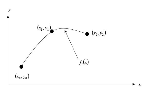
Figure 4 Quadratic interpolation.
Example 2
The upward velocity of a rocket is given as a function of time in Table 2.
Table 2 Velocity as a function of time.
| \(t\ (s)\) | \(v(t)\ (\text{m/s})\) |
|---|---|
| \(0\) | \(0\) |
| \(10\) | \(227.04\) |
| \(15\) | \(362.78\) |
| \(20\) | \(517.35\) |
| \(22.5\) | \(602.97\) |
| \(30\) | \(901.67\) |
Determine the value of the velocity at \(t = 16\) seconds using second order polynomial interpolation using Newton’s divided difference polynomial method.
Solution
For quadratic interpolation, the velocity is given by
\[v(t) = b_{0} + b_{1}(t - t_{0}) + b_{2}(t - t_{0})(t - t_{1})\]
Since we want to find the velocity at \(t = 16,\) and we are using a second order polynomial, we need to choose the three data points that are closest to \(t = 16\) that also bracket \(t = 16\) to evaluate it. The three points are \(t_{0} = 10,\) \(t_{1} = 15,\) and \(t_{2} = 20\).
Then
\[t_{0} = 10,\ v(t_{0}) = 227.04\]
\[t_{1} = 15,\ v(t_{1}) = 362.78\]
\[t_{2} = 20,\ v(t_{2}) = 517.35\]
gives
\[\begin{split} b_{0} &= v(t_{0})\\ &= 227.04 \end{split}\]
\[\begin{split} b_{1} &= \frac{v(t_{1}) - v(t_{0})}{t_{1} - t_{0}}\\ &= \frac{362.78 - 227.04}{15 - 10}\\ &= 27.148 \end{split}\]
\[\begin{split} b_{2} &= \frac{\displaystyle \frac{v(t_{2}) - v(t_{1})}{t_{2} - t_{1}} - \frac{v(t_{1}) - v(t_{0})}{t_{1} - t_{0}}}{t_{2} - t_{0}}\\ &= \frac{\displaystyle \frac{517.35 - 362.78}{20 - 15} - \frac{362.78 - 227.04}{15 - 10}}{20 - 10}\\ &= \frac{30.914 - 27.148}{10}\\ &= 0.37660 \end{split}\]
Hence
\[\begin{split} v(t) &= b_{0} + b_{1}(t - t_{0}) + b_{2}(t - t_{0})(t - t_{1})\\ &= 227.04 + 27.148(t - 10) + 0.37660(t - 10)(t - 15),\ 10 \leq t \leq 20 \end{split}\]
At \(t = 16,\)
\[\begin{split} v(16) &= 227.04 + 27.148(16 - 10) + 0.37660(16 - 10)(16 - 15)\\ &= 392.19\text{ m/s} \end{split}\]
If we expand
\[v(t) = 227.04 + 27.148(t - 10) + 0.37660(t - 10)(t - 15),\ 10 \leq t \leq 20\]
we get
\[v(t) = 12.05 + 17.733t + 0.37660t^{2},\ 10 \leq t \leq 20\]
This is the same expression obtained by the direct method.
General Form of Newton’s Divided Difference Polynomial
In the two previous cases, we found linear and quadratic interpolants for Newton’s divided difference method. Let us revisit the quadratic polynomial interpolant formula
\[f_{2}(x) = b_{0} + b_{1}(x - x_{0}) + b_{2}(x - x_{0})(x - x_{1})\]
where
\[b_{0} = f(x_{0})\]
\[b_{1} = \frac{f(x_{1}) - f(x_{0})}{x_{1} - x_{0}}\]
\[b_{2} = \frac{\displaystyle \frac{f(x_{2}) - f(x_{1})}{x_{2} - x_{1}} - \frac{f(x_{1}) - f(x_{0})}{x_{1} - x_{0}}}{x_{2} - x_{0}}\]
Note that \(b_0\), \(b_{1},\) and \(b_{2}\) are finite divided differences. \(b_0\), \(b_{1},\) and \(b_{2}\) are the first, second, and third finite divided differences, respectively. We denote the first divided difference by
\[f\lbrack x_{0}\rbrack = f(x_{0})\]
the second divided difference by
\[f\lbrack x_{1},x_{0}\rbrack = \frac{f(x_{1}) - f(x_{0})}{x_{1} - x_{0}}\]
and the third divided difference by
\[\begin{split} f\lbrack x_{2},x_{1},x_{0}\rbrack &= \frac{f\lbrack x_{2},x_{1}\rbrack - f\lbrack x_{1},x_{0}\rbrack}{x_{2} - x_{0}}\\ &= \frac{\displaystyle \frac{f(x_{2}) - f(x_{1})}{x_{2} - x_{1}} - \frac{f(x_{1}) - f(x_{0})}{x_{1} - x_{0}}}{x_{2} - x_{0}} \end{split}\]
where \(f\lbrack x_{0}\rbrack,f\lbrack x_{1},x_{0}\rbrack,\) and \(f\lbrack x_{2},x_{1},x_{0}\rbrack\) are called bracketed functions of their variables enclosed in square brackets.
Rewriting,
\[f_{2}(x) = f\lbrack x_{0}\rbrack + f\lbrack x_{1},x_{0}\rbrack(x - x_{0}) + f\lbrack x_{2},x_{1},x_{0}\rbrack(x - x_{0})(x - x_{1})\]
This leads us to writing the general form of the Newton’s divided difference polynomial for \(n + 1\) data points, \(\left( x_{0},y_{0} \right),\left( x_{1},y_{1} \right),\ldots\ldots,\left( x_{n - 1},y_{n - 1} \right),\left( x_{n},y_{n} \right)\), as
\(f_{n}(x) = b_{0} + b_{1}(x - x_{0}) + \ldots + b_{n}(x - x_{0})(x - x_{1})...(x - x_{n - 1})\)
where
\[b_{0} = f\lbrack x_{0}\rbrack\]
\[b_{1} = f\lbrack x_{1},x_{0}\rbrack\]
\[b_{2} = f\lbrack x_{2},x_{1},x_{0}\rbrack\]
\[\vdots\]
\[b_{n - 1} = f\lbrack x_{n - 1},x_{n - 2},\ldots,x_{0}\rbrack\]
\[b_{n} = f\lbrack x_{n},x_{n - 1},\ldots,x_{0}\rbrack\]
where the definition of the \(m^{\text{th}}\) divided difference is
\[\begin{split} b_{m} &= f\lbrack x_{m},\ldots\ldots,x_{0}\rbrack\\ &= \frac{f\lbrack x_{m},\ldots\ldots,x_{1}\rbrack - f\lbrack x_{m - 1},\ldots\ldots,x_{0}\rbrack}{x_{m} - x_{0}} \end{split}\]
From the above definition, it can be seen that the divided differences are calculated recursively.
For an example of a third order polynomial, given \((x_{0},y_{0}),\) \((x_{1},y_{1}),\) \((x_{2},y_{2}),\) and \((x_{3},y_{3}),\)
\[\begin{split} f_{3}(x)=f\left[x_{0}\right]&+f\left[x_{1}, x_{0}\right] \left(x-x_{0}\right)+f\left[x_{2}, x_{1}, x_{0}\right]\left(x-x_{0}\right)\left(x-x_{1}\right)\\ &+f\left[x_{3}, x_{2}, x_{1}, x_{0}\right]\left(x-x_{0}\right)\left(x-x_{1}\right)\left(x-x_{2}\right) \end{split}\]
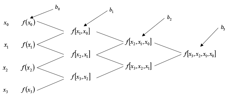
Figure 5 Table of divided differences for a cubic polynomial.
Example 3
The upward velocity of a rocket is given as a function of time in Table 3.
Table 3 Velocity as a function of time.
| \(t\ (s)\) | \(v(t)\ ({m/s})\) |
|---|---|
| \(0\) | \(0\) |
| \(10\) | \(227.04\) |
| \(15\) | \(362.78\) |
| \(20\) | \(517.35\) |
| \(22.5\) | \(602.97\) |
| \(30\) | \(901.67\) |
a) Determine the value of the velocity at \(t = 16\) seconds with third order polynomial interpolation using Newton’s divided difference polynomial method.
b) Using the third order polynomial interpolant for velocity, find the distance covered by the rocket from \(t = 11\text{ s}\) to \(t = 16\text{ s}\).
c) Using the third order polynomial interpolant for velocity, find the acceleration of the rocket at \(t = 16\text{ s}\).
Solution
a) For a third order polynomial, the velocity is given by
\[v(t) = b_{0} + b_{1}(t - t_{0}) + b_{2}(t - t_{0})(t - t_{1}) + b_{3}(t - t_{0})(t - t_{1})(t - t_{2})\]
Since we want to find the velocity at \(t = 16,\) and we are using a third order polynomial, we need to choose the four data points that are closest to \(t = 16\) that also bracket \(t = 16\) to evaluate it. The four data points are \(t_{0} = 10,\) \(t_{1} = 15,\) \(t_{2} = 20,\) and \(t_{3} = 22.5\).
Then
\[t_{0} = 10,\ v(t_{0}) = 227.04\]
\[t_{1} = 15,\ v(t_{1}) = 362.78\]
\[t_{2} = 20,\ v(t_{2}) = 517.35\]
\[t_{3} = 22.5,\ v(t_{3}) = 602.97\]
gives
\[\begin{split} b_{0} &= v\lbrack t_{0}\rbrack\\ &= v(t_{0})\\ &= 227.04 \end{split}\]
\[\begin{split} b_{1} &= v\lbrack t_{1},t_{0}\rbrack\\ &= \frac{v(t_{1}) - v(t_{0})}{t_{1} - t_{0}}\\ &= \frac{362.78 - 227.04}{15 - 10}\\ &= 27.148 \end{split}\]
\[\begin{split} b_{2} &= v\lbrack t_{2},t_{1},t_{0}\rbrack\\ &= \frac{v\lbrack t_{2},t_{1}\rbrack - v\lbrack t_{1},t_{0}\rbrack}{t_{2} - t_{0}} \end{split}\]
\[\begin{split} v\lbrack t_{2},t_{1}\rbrack &= \frac{v(t_{2}) - v(t_{1})}{t_{2} - t_{1}}\\ &= \frac{517.35 - 362.78}{20 - 15}\\ &= 30.914 \end{split}\]
\[v\lbrack t_{1},t_{0}\rbrack = 27.148\]
\[\begin{split} b_{2} &= \frac{v\lbrack t_{2},t_{1}\rbrack - v\lbrack t_{1},t_{0}\rbrack}{t_{2} - t_{0}}\\ &= \frac{30.914 - 27.148}{20 - 10}\\ &= 0.37660 \end{split}\]
\[\begin{split} b_{3} &= v\lbrack t_{3},t_{2},t_{1},t_{0}\rbrack\\ &= \frac{v\lbrack t_{3},t_{2},t_{1}\rbrack - v\lbrack t_{2},t_{1},t_{0}\rbrack}{t_{3} - t_{0}} \end{split}\]
\[v\lbrack t_{3},t_{2},t_{1}\rbrack = \frac{v\lbrack t_{3},t_{2}\rbrack - v\lbrack t_{2},t_{1}\rbrack}{t_{3} - t_{1}}\]
\[\begin{split} v\lbrack t_{3},t_{2}\rbrack &= \frac{v(t_{3}) - v(t_{2})}{t_{3} - t_{2}}\\ &= \frac{602.97 - 517.35}{22.5 - 20}\\ &= 34.248 \end{split}\]
\[\begin{split} v\lbrack t_{2},t_{1}\rbrack &= \frac{v(t_{2}) - v(t_{1})}{t_{2} - t_{1}}\\ &= \frac{517.35 - 362.78}{20 - 15}\\ &= 30.914 \end{split}\]
\[\begin{split} v\lbrack t_{3},t_{2},t_{1}\rbrack &= \frac{v\lbrack t_{3},t_{2}\rbrack - v\lbrack t_{2},t_{1}\rbrack}{t_{3} - t_{1}}\\ &= \frac{34.248 - 30.914}{22.5 - 15}\\ &= 0.44453 \end{split}\]
\[v\lbrack t_{2},t_{1},t_{0}\rbrack = 0.37660\]
\[\begin{split} b_{3} &= \frac{v\lbrack t_{3},t_{2},t_{1}\rbrack - v\lbrack t_{2},t_{1},t_{0}\rbrack}{t_{3} - t_{0}}\\ &= \frac{0.44453 - 0.37660}{22.5 - 10}\\ &= 5.4347 \times 10^{- 3} \end{split}\]
Hence
\[\begin{split} v(t) &= b_{0} + b_{1}(t - t_{0}) + b_{2}(t - t_{0})(t - t_{1}) + b_{3}(t - t_{0})(t - t_{1})(t - t_{2})\\ &=227.04+27.148(t-10)+0.37660(t-10)(t-15)\\ & \ \ \ \ + 5.5347 \times 10^{- 3}(t - 10)(t - 15)(t - 20) \end{split}\]
At \(t = 16,\) \[\begin{split} v(16)&=227.04+27.148(16-10)+0.37660(16-10)(16-15)\\ & \ \ \ \ + 5.5347 \times 10^{- 3}(16 - 10)(16 - 15)(16 - 20)\\ &= 392.06{\ m/s} \end{split}\]
b) The distance covered by the rocket between \(t = 11\text{ s}\) and \(t = 16\text{ s}\) can be calculated from the interpolating polynomial
\[\begin{split} v(t) &= 227.04 + 27.148(t - 10) + 0.37660(t - 10)(t - 15)\\ & \ \ \ \ +5.5347\times10^{-3}(t-10)(t-15)(t-20)\\ &= - 4.2541 + 21.265t + 0.13204t^{2} + 0.0054347t^{3},\ 10 \leq t \leq 22.5 \end{split}\]
Note that the polynomial is valid between \(t = \text{10}\) and \(t = \text{22.5}\) and hence includes the limits of \(t = 11\) and \(t = 16\).
So
\[\begin{split} s(16) - s(11) &= \int_{11}^{16}{v(t){dt}}\\ &= \int_{11}^{16}( - 4.2541 + 21.265t + 0.13204t^{2} + 0.0054347t^{3}){dt}\\ &= \left\lbrack - 4.2541t + 21.265\frac{t^{2}}{2} + 0.13204\frac{t^{3}}{3} + 0.0054347\frac{t^{4}}{4} \right\rbrack_{11}^{16}\\ &= 1605{\ m} \end{split}\]
c) The acceleration at \(t = 16\) is given by
\[ a(16)=\left.\frac{d}{d t} v(t)\right|_{t=16}\] \[\begin{split} a(t) &= \frac{d}{{dt}}v(t)\\ &= \frac{d}{{dt}}\left( - 4.2541 + 21.265t + 0.13204t^{2} + 0.0054347t^{3} \right)\\ &= 21.265 + 0.26408t + 0.016304t^{2} \end{split}\]
\[\begin{split} a(16) &= 21.265 + 0.26408(16) + 0.016304(16)^{2}\\ &= 29.664{\ m/}{s}^{2} \end{split}\]
Multiple Choice Test
(1). If a polynomial of degree \(n\) has more than \(n\) zeros, then the polynomial is
(A) oscillatory
(B) zero everywhere
(C) quadratic
(D) not defined
(2). The following \(x\) -\(y\) data is given.
| \(x\) | \(15\) | \(18\) | \(22\) |
| \(y\) | \(24\) | \(37\) | \(25\) |
The Newton’s divided difference second order polynomial for the above data is given by
\[f_{2}(x) = b_{0} + b_{1}\left( x - 15 \right) + b_{2}\left( x - 15 \right)\left( x - 18 \right)\]
The value of \(b_{1}\) is most nearly
(A) \(-1.0480\)
(B) \(0.14333\)
(C) \(4.3333\)
(D) \(24.000\)
(3). The polynomial that passes through the following \(x\) -\(y\) data
| \(x\) | \(18\) | \(22\) | \(24\) |
| \(y\) | \(?\) | \(25\) | \(123\) |
is given by
\[8.125x^{2} - 324.75x + 3237,\ 18 \leq x \leq 24\]
The corresponding polynomial using Newton’s divided difference polynomial is given by
\[f_{2}(x) = b_{0} + b_{1}\left( x - 18 \right) + b_{2}\left( x - 18 \right)\left( x - 22 \right)\]
The value of \(b_{2}\) is
(A) \(0.25000\)
(B) \(8.1250\)
(C) \(24.000\)
(D) not obtainable with the information given
(4). Velocity vs. time data for a body is approximated by a second order Newton’s divided difference polynomial as
\[v\left( t \right) = b_{0} + 39.622\left( t - 20 \right) + 0.5540\left( t - 20 \right)\left( t - 15 \right),{\ \ }10 \leq t \leq 20\]
The acceleration in \({m/}{s}^{2}\) at \(t = 15\) is
(A) \(0.55400\)
(B) \(39.622\)
(C) \(36.852\)
(D) not obtainable with the given information
(5). The path that a robot is following on a x-y plane is found by interpolating four data points as
| \(x\) | \(2\) | \(4.5\) | \(5.5\) | \(7\) |
| \(y\) | \(7.5\) | \(7.5\) | \(6\) | \(5\) |
\[y\left( x \right) = 0.15238x^{3} - 2.2571x^{2} + 9.6048x - 3.9000\]
The length of the path from \(x = 2\) to \(x = 7\) is
(A) \(\displaystyle \sqrt{\left( 7.5 - 7.5 \right)^{2} + \left( 4.5 - 2 \right)^{2}} + \sqrt{\left( 6 - 7.5 \right)^{2} + \left( 5.5 - 4.5 \right)^{2}} + \sqrt{\left( 5 - 6 \right)^{2} + \left( 7 - 5.5 \right)^{2}}\)
(B) \(\displaystyle \int_{2}^{7}\sqrt{1 + (0.15238x^{3} - 2.2571x^{2} + 9.6048x - 3.9000)^{2}}{dx}\)
(C) \(\displaystyle \int_{2}^{7}\sqrt{1 + (0.45714x^{2} - 4.5142x + 9.6048)^{2}}{dx}\)
(D) \(\displaystyle \int_{2}^{7}{(0.15238x^{3} - 2.2571x^{2} + 9.6048x - 3.9000)}{dx}\)
(6). The following data of the velocity of a body is given as a function of time.
| Time \((s)\) | \(0\) | \(15\) | \(18\) | \(22\) | \(24\) |
| Velocity \((m/s)\) | \(22\) | \(24\) | \(37\) | \(25\) | \(123\) |
If you were going to use quadratic interpolation to find the value of the velocity at \(t = 14.9\) seconds, the three data points of time you would choose for interpolation are
(A) \(0, 15, 18\)
(B) \(15, 18, 22\)
(C) \(0, 15, 22\)
(D) \(0, 18, 24\)
For complete solution, go to
http://nm.mathforcollege.com/mcquizzes/05inp/quiz_05inp_newton_solution.pdf
Problem Set
(1). The following data of the velocity of a body as a function of time is given
| \(\text{Time}\ (s)\) | \(0\) | \(15\) | \(18\) | \(22\) | \(24\) |
|---|---|---|---|---|---|
| \(\text{Velocity}\ (m/s)\) | \(22\) | \(24\) | \(37\) | \(25\) | \(123\) |
Find the coefficients of the Newton’s divided difference interpolating first order polynomial to find the velocity at \(t = 14\ \text{s}\).
Answer: \(\text{velocity at}\ 14\ \text{seconds} = 23.867\ \text{m/s}\)
(2). The following data of the velocity of a body as a function of time is given
| \(\text{Time}\ (s)\) | \(0\) | \(15\) | \(18\) | \(22\) | \(24\) |
|---|---|---|---|---|---|
| \(\text{Velocity}\ (m/s)\) | \(22\) | \(24\) | \(37\) | \(25\) | \(123\) |
Find the coefficients of the Newton’s divided difference interpolating second order polynomial to find the velocity at \(t = 14\ \text{s}\).
Answer: \(\text{velocity at}\ 14\ \text{seconds} = 20.6\ \text{m/s}\)
(3). The following data of the velocity of a body as a function of time is given
| \(\text{Time}\ (s)\) | \(0\) | \(15\) | \(18\) | \(22\) | \(24\) |
|---|---|---|---|---|---|
| \(\text{Velocity}\ (m/s)\) | \(22\) | \(24\) | \(37\) | \(25\) | \(123\) |
Find the coefficients of the Newton’s divided difference interpolating third order polynomial to find the velocity at \(t = 14\ \text{s}\).
Answer: \(\text{velocity at}\ 14\ \text{seconds} = 17.339\ \text{m/s}\)
(4). You are given data for the upward velocity of a rocket as a function of time in the table below.
| \(t,\ (s)\) | \(0\) | \(10\) | \(15\) | \(20\) | \(22.5\) | \(30\) |
|---|---|---|---|---|---|---|
| \(v(t),\ (m/s)\) | \(0\) | \(227.04\) | \(362.78\) | \(517.35\) | \(602.97\) | \(901.67\) |
a) Use Newton’s divided difference linear interpolant approximation of velocity to find the acceleration at \(t = 16\ \text{s}\).
b) Use Newton’s divided difference quadratic interpolant approximation of velocity to find the acceleration at \(t = 16\ \text{s}\).
c) Find the distance covered by the rocket from \(t = 5\ \text{s}\) to \(16\ \text{s}\)? Use any method.
Answer: \(a)\ a(16) = 30.914 \ \text{m/s}^2 \ \ b)\ a(16) = 29.784\ \text{m/s}^2\)
(5). The acceleration-time data for a small rocket is given in tabular form below.
| \(\text{Time}\ (s)\) | \(10\) | \(12\) | \(14\) | \(16\) | \(18\) | \(20\) | \(22\) | \(24\) |
|---|---|---|---|---|---|---|---|---|
| \(\text{Acceleration}\ m/s^2\) | \(106.6\) | \(94.1\) | \(80.9\) | \(68.0\) | \(56.2\) | \(45.8\) | \(37.1\) | \(30.1\) |
a) Use Newton’s divided difference quadratic polynomial interpolation to find the acceleration at \(t = 15.5\) seconds. Be sure to choose your base points for good accuracy.
b) Use the quadratic interpolant of part (a) to find the change in the velocity of the rocket between \(t = 14.1\) and \(t = 15.8\) seconds.
Answer: \(a)\ a(15.5) = 71.122\ \text{m/s}^2\ \ b)\ \text{Change in velocity} = 126.94 \ \text{m/s}\)
(6). A robot follows a path generated by a quadratic interpolant from x = 2 to x = 4. The interpolant passes through three consecutive data points \((2,4),\ (3,9)\) and \((4,16)\) and is given by \(y = x^{2}\). Find the length of the interpolant path from \(x = 2\) to \(x = 4\). You can approximate a general integral by
\[\int_{a}^{b}{f(x)dx} \approx \frac{(b - a)}{6}\left\lbrack f(a) + 4f\left( \frac{a + b}{2} \right) + f(b) \right\rbrack\]
Answer: \(\text{Length} = 12.172\)