Chapter 03.00: Physical Problem for Nonlinear Equations
Summary
Finding the depth to which a ball would float in water requires solving a nonlinear equation.
Modeling
You are working for ‘DOWN THE TOILET COMPANY’ that makes floats for ABC commodes. The ball has a specific gravity of 0.6 and has a radius of 5.5 cm. You are asked to find the depth to which the ball will get submerged when floating in water (see Figure 1).
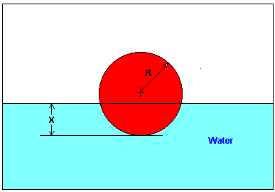
Figure 1 Depth to which the ball is submerged in water
According to Newton’s third law of motion, every action has an equal and opposite reaction. In this case, the weight of the ball is balanced by the buoyancy force (Figure 2).
\[\text{Weight of ball} = \text{Buoyancy force} \;\;\;\;\;\;\;\;\;\;\;\; (1)\]
The weight of the ball is given by
\[\begin{split} \text{Weight of ball} &= \text{(Volume of ball)} \times \text{(Density of ball)} \times \text{(Acceleration due to gravity)}\\ &=\left( \frac{4}{3}\pi R^{3} \right)\left( \rho_{b} \right)\left( g \right)\;\;\;\;\;\;\;\;\;\;\;\; (2) \end{split}\]
where
\[R = \text{radius of the ball}\ (\text{m}),\]
\[\rho = \text{density of the ball}\ \left( \text{kg/m}^{3} \right),\]
\[g = \text{acceleration due to gravity}\ \left(\text{m/s}^{2} \right).\]
The buoyancy force is given by
\[\begin{split} \text{Buoyancy force} &= \text{Weight of water displaced}\\ &= \text{(Volume of the ball under water) (Density of water)(Acceleration due to gravity)}\\ &=\pi x^{2}\left( R - \frac{x}{3} \right)\rho_{w}g \;\;\;\;\;\;\;\;\;\;\;\; (3) \end{split}\]
where
\[x = \text{depth to which ball is submerged,}\]
\[\rho_{w} = \text{density of water.}\]
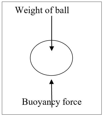
Figure 2 Free Body Diagram showing the forces acting on the ball immersed in water
Now substituting Equations (2) and (3) in Equation (1),
\[\frac{4}{3}\pi R^{3}\rho_{b}g = \pi x^{2}\left( R - \frac{x}{3} \right)\rho_{w}g\]
\[4R^{3}\rho_{b} = 3x^{2}(R - \frac{x}{3})\rho_{w}\]
\[4R^{3}\rho_{b} - 3x^{2}R\rho_{w} + x^{3}\rho_{w} = 0\]
\[4R^{3}\frac{\rho_{b}}{\rho_{w}} - 3x^{2}R + x^{3} = 0\]
\[4R^{3}\gamma_{b} - 3x^{2}R + x^{3} = 0 \;\;\;\;\;\;\;\;\;\;\;\; (4)\]
where
the specific gravity of the ball, \(\gamma_{b}\) is given by
\[\gamma_{b} = \frac{\rho_{b}}{\rho_{w}} \;\;\;\;\;\;\;\;\;\;\;\; (5)\]
Given
\[R = 5.5\ \text{cm} = 0.055\ \text{m},\]
\[\gamma_{b} = 0.6,{and}\]
substituting in Equation (4), we get
\[4(0.055)^{3}(0.6) - 3x^{2}(0.055) + x^{3} = 0\]
\[3.993 \times 10^{- 4} - 0.165x^{2} + x^{3} = 0\;\;\;\;\;\;\;\;\;\;\;\; (6)\]
Equation (6) is nonlinear. Solving it would give us the value of \(x\), that is, the depth to which the ball is submerged underwater.
Appendix: Derivation of the formula for the volume of a ball submerged underwater
How do you find that the volume of the ball submerged underwater as given by
\[V = \frac{\pi h^{2}\left( 3r - h \right)}{3}\;\;\;\;\;\;\;\;\;\;\;\; (7)\]
where
\[r = \text{radius of the ball,}\]
\[h = \text{height of the ball to which the ball is submerged.}\]
From calculus,
\[V = \int_{r - h}^{r}{Adx}\;\;\;\;\;\;\;\;\;\;\;\; (8)\]
where \(A\) is the cross-sectioned area at a distance \(x\) from the center of the sphere. The lower limit of integration is \(x = r - h\) as that is where the water line is
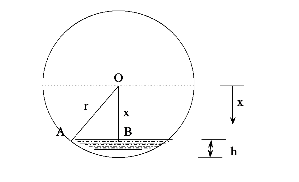
Figure 3 Deriving the equation for the volume of ball underwater
and the upper limit is \(r\) as that is the bottom of the sphere. So, what is the A at any location \(x\).
From Figure 3, for a location \(x\),
\[OB = x\]
\[OA = r,\]
then \[\begin{split} AB &= \sqrt{OA^{2} - OB^{2}}\\ &= \sqrt{r^{2} - x^{2}}\;\;\;\;\;\;\;\;\;\;\;\; (9) \end{split}\]
and AB is the radius of the area at \(x\). So at location \(B\) is
\[A = \pi(AB)^{2} = \pi\left( r^{2} - x^{2} \right)\;\;\;\;\;\;\;\;\;\;\;\; (10)\]
so
\[\begin{split} V &= \int_{r - h}^{r}{\pi\left( r^{2} - x^{2} \right){dx}}\\ &= \pi\left( r^{2}x - \frac{x^{3}}{3} \right)_{r - h}^{r}\\ &= \pi\left\lbrack \left( r^{2}r - \frac{r^{3}}{3} \right) - \left( r^{2}\left( r - h \right) - \frac{\left( r - h \right)^{3}}{3} \right) \right\rbrack\\ &= \frac{\pi h^{2}\left( 3r - h \right)}{3}.\;\;\;\;\;\;\;\;\;\;\;\; (11) \end{split}\]
Summary
Designing a scale to find the volume of oil in a spherical tank requires solving a nonlinear equation.
Modeling
Years ago, a businessperson called me and wanted to know how he could find how much oil was left in his storage tank. His tank was spherical and was 6 feet in diameter. Well, I suggested him to get a 8ft steel ruler and use it as a dipstick (Figure 1). Knowing the height
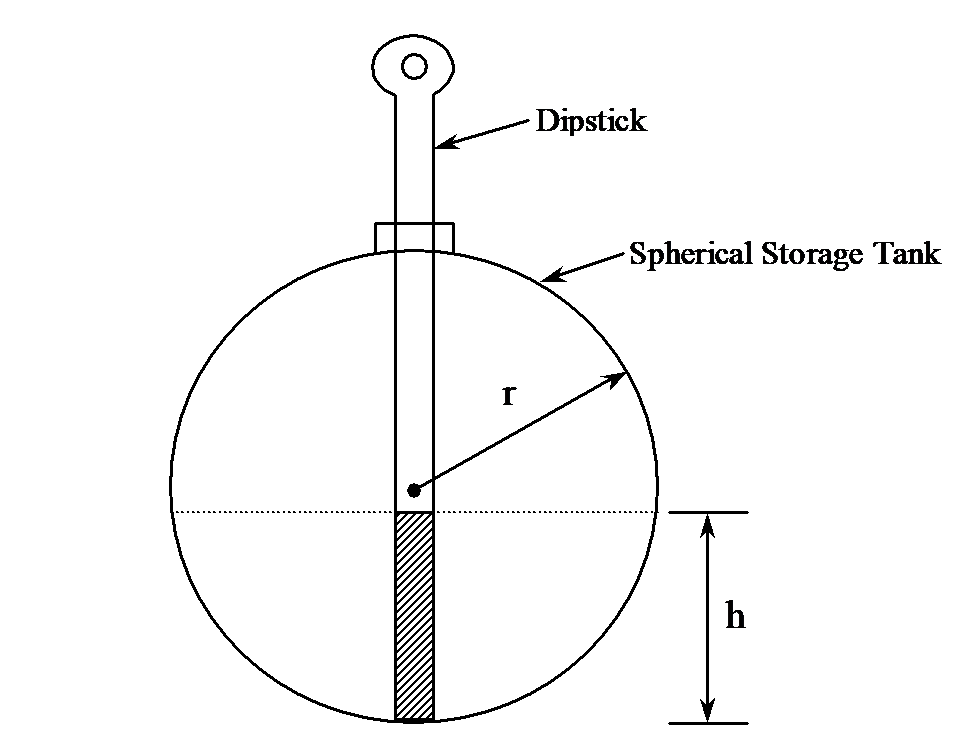
Figure 1 Oil in a spherical storage tank.
to which the dip-stick would become wet with oil, one would know the height \(h\) of the oil in the tank. The volume \(V\) of oil left in the tank then is
\[V = \frac{\pi h^{2}\left( 3r - h \right)}{3} \ \ \ (1)\]
where, \(r\) is the radius of the tank. But, he did not stop there. He wanted me to design a steel ruler for him so that he would directly get the reading from the dipstick. How would I design such a dipstick?
The problem is inverse of what he wanted originally. To design a dipstick, I would have to mark the height corresponding to a volume. To do that I would need to solve the equation
\[V = \frac{\pi h^{2}\left( 3r - h \right)}{3}\]
for the height for a given volume and radius. For example, where would you mark the scale for \(4ft^{3}\) of oil?
\[4 = \frac{\pi h^{2}\left( 3 \times 3 - h \right)}{3}\]
\[h^{3} - 9h^{2} + \frac{12}{\pi} = 0\]
\[f\left( h \right) = h^{3} - 9h^{2} + 3.8197 = 0\]
Therefore, this nonlinear equation needs to be solved. To mark the scale for other volumes, you will need to substitute the value for the volume and solve for \(h\). Continue to do this for different preset volumes to develop the scale.
Appendix A: Derivation of the formula for the volume of the oil based on radius of the tank and the height of oil in the tank
How do you find that the volume of oil is given by
\[V = \frac{\pi h^{2}\left( 3r - h \right)}{3}\]
From calculus,
\[V = \int_{r - h}^{r}{Adx}\]
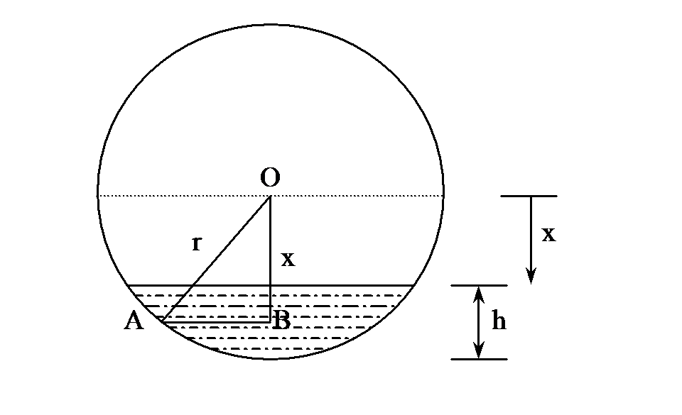
Figure 2 Deriving the equation for volume of oil in the tank.
where \(A\) is the cross-sectioned area at the location \(x\), from the center of the sphere. The lower limit of integration is \(x = r - h\)as that is where the oil line is and the upper limit is \(r\) as that is the bottom of the sphere. So, what is \(A\) at any location \(x\)?
From Figure 2, for a location \(x\)
\[OB = x\]
\[OA = r\]
then
\[\begin{split} AB &= \sqrt{OA^{2} - OB^{2}}\\ &= \sqrt{r^{2} - x^{2}} \end{split}\]
and \({AB}\) is the radius of the area at \(x\). So the area at location \(x\) is
\[\begin{split} A &= \pi(AB)^{2}\\ &= \pi\left( r^{2} - x^{2} \right) \end{split}\]
So
\[\begin{split} V &= \int_{r - h}^{r}{\pi\left( r^{2} - x^{2} \right){dx}}\\ &=pi\left( r^{2}x - \frac{x^{3}}{3} \right)_{r - h}^{r}\\ &= \pi\left\lbrack \left( r^{2}r - \frac{r^{3}}{3} \right) - \left( r^{2}\left( r - h \right) - \frac{\left( r - h \right)^{3}}{3} \right) \right\rbrack\\ &= \frac{\pi h^{2}\left( 3r - h \right)}{3}. \end{split}\]
Modeling
My spouse asked me to build a bookshelf (Figure 1) for her books. Her books range from \(8\frac{1}{2}^{\prime\prime}\) in to \(11^{\prime\prime}\) in height, and would take \(29^{\prime\prime}\) of space along the length. She asked me how much would the bookshelf sag, as she does not like sagging bookshelves we had during graduate student days. After all, our tolerance to sagging does sag after graduation! So, as a true engineer, before going to the local building store, I modeled the problem to find the maximum deflection of the bookshelf. I assumed a shelf of thickness \(3/8^{\prime\prime}\) and width \(12^{\prime\prime}\). The Young’s modulus of a typical wood shelf material is 3.667 Msi.
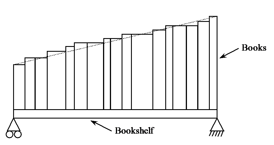
Figure 1 Distributions of books on the bookshelf.
I assume the following
100 pages of \(8\frac{1}{2}^{\prime\prime} \times 11^{\prime\prime}\) book paper weighs 1 lb (on its website www.usps.gov, United States Post Office suggests 6 letter size pages weigh about 1 ounce, so 100 pages would be approximately a pound).
400 pages take up the space of \(1^{\prime\prime}\) in thickness (I actually measured several textbooks and found an average.)
the books decrease linearly in height from \(11^{\prime\prime}\) from the right end to \(8\frac{1}{2}^{\prime\prime}\) on the left, and the book width is \(8\frac{1}{2}^{\prime\prime}\) for all books,
The total weight \(W\) of the books is found as follows. If all the books were of dimensions \(11^{\prime\prime} \times 8\frac{1}{2}^{\prime\prime}\), the weight of the books would be
\[\begin{split} W &= 29{in} \times 400\frac{{pages}}{{in}}\ \times \ \frac{1{lb}}{100{pages}}\\ &= 116 lb \end{split}\]
But since the books decrease in height from \(11^{\prime\prime}\) to \(8\frac{1}{2}^{\prime\prime}\), while the width of the books is assumed to be constant at \(8\frac{1}{2}^{\prime\prime}\), the actual total weight of the books is calculated as
\[\begin{split} W &= \frac{\frac{1}{2}\left( 11 + 8\frac{1}{2} \right)29}{\left( 11 \right)\left( 29 \right)} \times 116\\ &\approx 103{lb}\\ \end{split}\]
Now assuming that the weight ‘\(W\)’ is distributed linearly from the left end to the right as a distribution \(q\) (Figure 2),
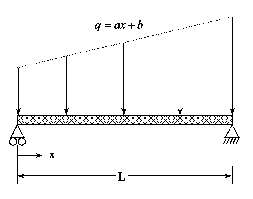
Figure 2 Approximate weight distribution of books.
Then the total weight \(W\) over the length \(L\)
\[\begin{split} W &= \int_{0}^{L}{qdx}\\ &= \int_{0}^{L}{\left( ax + b \right){dx}}\\ &= a\frac{L^{2}}{2} + bL \ \ \ (1) \end{split}\]
Also, the weight distribution can be assumed to be in the same ratio as the height of the books at the two ends, then
\[\frac{q\left( x = 0 \right)}{q\left( x = L \right)} = \frac{8.5}{11}\]
\[\frac{a\left( 0 \right) + b}{aL + b} = \frac{8.5}{11}\]
\[\frac{b}{aL + b} = \frac{8.5}{11}\ \ \ (2)\]
Substituting
\[W = 103{lb},\]
\[L = 29^{\prime\prime},\]
in Equations (1) and (2), we get
\[a\frac{29^{2}}{2} + b\left( 29 \right) = 103\]
\[\frac{b}{a\left( 29 \right) + b} = \frac{8.5}{11}\]
or
\[420.5a + 29b = 103\]
\[- 246.5a + 3b = 0\]
The above set of equations gives the solution as
\[a = 0.031403\]
\[b = 3.0964\]
So the weight distribution is given by
\[q = 0.031403x + 3.0964,\ 0 \leq x \leq 29\]
Now let us find the deflection in the beam. The deflection \(y\) as a function of \(x\) along the length of the beam is given by
\[\frac{d^{2}y}{dx^{2}} = \frac{M}{EI}\]
where
\[M = \text{Bending moment}\ \left({lb.in} \right)\]
\[E = \text{Young's modulus}\ \left({psi} \right)\]
\[I = \text{Second moment of area}\ \left( in^{4} \right)\]
To find the bending moment, we need to first find the reaction force at the support. Let \(R_{1}\) and \(R_{2}\) be the reactions at the left and right support, respectively (Figure 3). Then from the sum of forces in the vertical direction,
\[R_{1} + R_{2} = W\]
and the moment at the left support is zero as it is simply supported
\[R_{2}L - \int_{0}^{L}{\left( ax + b \right)xdx = 0}\]
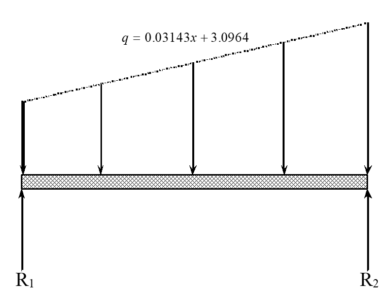
Figure 3 Reaction at the end of shelf supports.
\[ R_{2}L - a\frac{L^{3}}{3} - \frac{bL^{2}}{2} = 0\]
Substituting
\[W = 103,\]
\[a = 0.031403,\]
\[b = 3.0964,\]
\[L = 29,\]
the equilibrium equations are
\[R_{1} + R_{2} = 103\]
\[R_{2}\left( 29 \right) - \left( 0.031403 \right)\frac{29^{3}}{3} - 3.0964\frac{29^{2}}{2} = 0\]
gives
\[R_{1} = 49.300\ lb\]
\[R_{2} = 53.701\ lb\]
The bending moment at any cross-section at a distance of \(x\) from the left end is then given by summing the moments at a cross-section of distance \(x\) from the left end as (Figure 4)
\[M\left( x \right) - R_{1}x + \int_{0}^{L}{\left( ax^{'} + b \right)\left( x - x^{'} \right)dx^{'} = 0}\]
\[\begin{split} M\left( x \right) &= R_{1}x\int_{0}^{L}{\left( ax^{'} + b \right)\left( x - x^{\prime} \right)dx^{\prime}} \\ &= R_{1}x - \frac{1}{6}ax^{3} - \frac{1}{2}bx^{2} \end{split}\]
Substituting value of\(R_{1},a\) and \(b\),
\[R_{1} = 49.299\]
\[a = 0.031403\]
\[b = 3.0964\]
the bending moment equation is given by
\[M\left( x \right) = 49.299x - \frac{1}{6}\left( 0.031403 \right)x^{3} - \frac{1}{2}\left( 3.0964 \right)x^{2}\]
\[M\left( x \right) = 49.299x - 0.0052339x^{3} - 1.5482x^{2}\]
So
\[{EI}\frac{d^{2}v}{dx^{2}} = M\left( x \right)\]
\[\frac{d^{2}v}{dx^{2}} = \frac{M\left( x \right)}{{EI}}\]
\[E = 3.667Msi\]
\[I = \frac{1}{12}ht^{3}\]
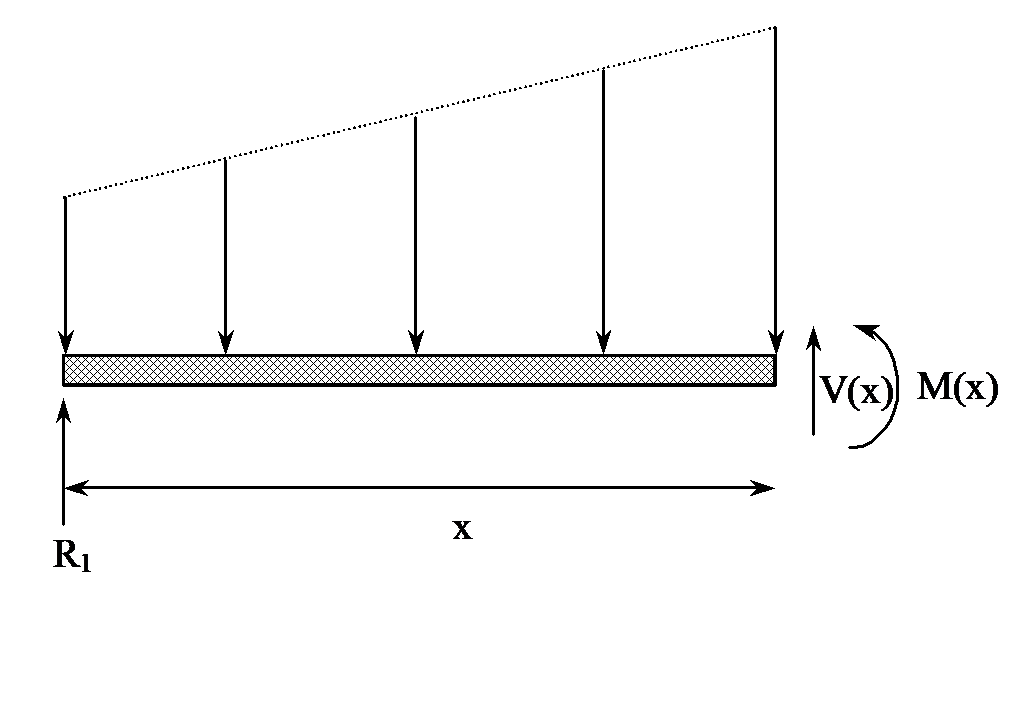
Figure 4 Free body diagram to find bending moment at a cross-section.
where
\[h = \text{width of shelf}\]
\[t = \text{thickness of shelf}\]
\[\begin{split} I &= \frac{1}{12} \times 12 \times \left( \frac{3}{8} \right)^{3}\\ &= 0.052734{in} \end{split}\]
Hence
\[\begin{split} \frac{d^{2}v}{dx^{2}} &= \frac{M\left( x \right)}{{EI}}\\ &= \frac{49.29x - 0.0052339x^{3} - 1.5428x^{2}}{3.6667 \times 10^{6} \times 0.052734}\\ &= 0.25496 \times 10^{- 3}x - 0.27068 \times 10^{- 7}x^{3} - 0.80067 \times 10^{- 5}x^{2} \end{split}\]
Integrating with respect to \(x\) gives
\[\frac{{dv}}{{dx}} = 0.25496 \times 10^{- 3}x^{2} - 0.67670 \times 10^{- 8}x^{4} - 0.26689 \times 10^{- 5}x^{3} + c_{1}\]
Integrating once again with respect to \(x\) gives
\[ v\left( x \right) = 0.42493 \times 10^{- 4}x^{3} - 0.13534 \times 10^{- 8}x^{5} - 0.66723 \times 10^{- 6}x^{4} + c_{1}x + c_{2}\]
Now the boundary conditions at \(x = 0\) and \(x = L\) are that the displacement is zero at the ends,
\[v\left( 0 \right) = 0\]
\[v\left( L \right) = 0\]
So from
\[v\left( 0 \right) = 0\]
we get
\[c_{2} = 0,\ \text{and}\]
from
\[v(L) = 0\]
we get
\[0 = 0.42493 \times 10^{- 3}L^{3} - 0.13534 \times 10^{- 8}L^{5} - 0.66723 \times 10^{- 6}L^{4} + c_{1}L\]
Substituting \(L = 29^{\prime\prime}\)
\[0 = 0.42493 \times 10^{- 3}\left( 29 \right)^{3} - 0.13534 \times 10^{- 8}\left( 29 \right)^{5} - 0.66723 \times 10^{- 6}\left( 29 \right)^{4} + c_{1}\left( 29 \right)\]
\[c_{1} = - 0.018506\]
Hence the vertical deflection in the beam is given by
\[v\left( x \right) = 0.42493 \times 10^{- 4}x^{3} - 0.13534 \times 10^{- 8}x^{5} - 0.66723 \times 10^{- 6}x^{4} - 0.018506x\]
But to find where the deflection would be maximum, we need to take the first derivative of the deflection to find where
\[\frac{{dv}}{{dx}} = 0,\]
that is
\[\frac{d}{{dx}}(0.42493 \times 10^{- 4}x^{3} - 0.13534 \times 10^{- 8}x^{5} - 0.66723 \times 10^{- 6}x^{4} - 0.018506x) = 0\]
\[f(x) = 0.12748 \times 10^{- 3}x^{2} - 0.67670 \times 10^{- 8}x^{4} - 0.26689 \times 10^{- 5}x^{3} - 0.018506 = 0\]
Now here is a nonlinear equation that needs to solved to find where the maximum deflection occurs. Then substituting the obtained value of \(x\) in \(v\left( x \right)\) would give us the maximum sagging in the beam.
Summary
For efficient design of the Cray supercomputer, it does not have a divide unit. It uses a numerical solution of a nonlinear equation to find the inverse of a number.
Modeling
Many super computers do not have a unit to divide numbers. But why? Well, a divide operation in modern computers can take 20 to 25 clock cycles, and that is five times what it takes for multiplication [1]. Instead, a divide unit, based on numerically solving a nonlinear equation, is developed. This allows for a faster divide operation. This is how it works.
If you want to find the value of \(b/a\) where \(b\) and \(a\) are real numbers, one can look at
\[\frac{b}{a} = b*\frac{1}{a} = b*c\]
where
\[c = \frac{1}{a}\]
So, if one is able to find \(c\), we only need to multiply \(b\) and \(c\) to find \(b/a\). So how do we find \(c\) without the divide unit.
Equation
\[c = \frac{1}{a}\]
can be written as an equation
\[f\left( c \right) = ac - 1 = 0\]
If one is able to find the root of this equation without using a division, then we have the value of \(1/a\).
Although we do not explain the numerical methods of solving nonlinear equations in this section of the notes, it becomes necessary to do so in this example. The Newton-Raphson method of solving a nonlinear equation is used in finding \(1/a\). The Newton Raphson method of solving an equation \(f\left( c \right) = 0\) is given by the iterative formula
\[c_{i + 1} = c_{i} - \frac{f\left( c_{i} \right)}{f'\left( c_{i} \right)},\]
where
\[c_{i + 1}\ \text{is the new approximation of of the root of}\ f(c) = 0\ \text{and}\]
\[c_{i}\ \text{is the previous approximation of the root of}\ f(c) = 0.\]
What is the appropriate function to use to find the inverse of \(\mathbf{a}\)?
a) Using
\[f\left( c \right) = ac - 1 = 0\]
gives
\[f^\prime\left( c \right) = a\]
and the Newton-Raphson method formula gives
\[c_{i + 1} = c_{i} - \frac{ac_{i} - 1}{a}\]
\[c_{i + 1} = \frac{1}{a}\]
This is of no use as it involves division.
b) Using
\[f\left( c \right) = a - \frac{1}{c} = 0\]
gives
\[f^\prime \left( c \right) = \frac{1}{c^{2}}\]
\[\begin{split} c_{i + 1} &= c_{i} - \frac{\displaystyle a - \frac{1}{c_{i}}}{\displaystyle \frac{1}{c_{i}^{2}}}\\ &= c_{i} - c_{i}^{2}\left( a - \frac{1}{c_{i}} \right) \end{split}\]
\[c_{i + 1} = c_{i}\left( 2 - c_{i}a \right)\]
This one is the acceptable iterative formula to find the inverse of \(a\) as it does not involve division.
Starting with an initial guess for the inverse of \(a\), one can find newer approximations by using the above iterative formula. Each iteration requires two multiplications and one subtraction. However, the number of iterations required to find the inverse of \(a\) very much depends on the initial approximation. More accurate is the starting approximation, less number of iterations are required to find the inverse of \(a\). Since the convergence of Newton Raphson method is quadratic, it may take up to six iterations to get an accurate reciprocal in double precision. By using look-up tables for the initial approximation, the number of iterations required can be reduced to two [2]. Also, the operation of \(\left( 2 - c_{i}a \right)\) may be carried in a fused multiply-subtract unit to further reduce the clock cycles needed for the computation.
References
1. Oberman, S.F., Flynn, M.J., “Division Algorithms and Implementations”, IEEE Transactions on Computers, Vol. 46, No. 8, 1997.
2. Wong, D., Flynn, M.J., “Fat Division using accurate quotient approximations to reduce the number of iteratoimns”, IEEE Transactions on Computers, Vol. 41, No. 8, 981-995, 1992.
Appendix A
Example of using Newton–Raphson method to find the inverse of a number
Let us find \(\displaystyle \frac{1}{2.5}\)
The Newton –Raphson method formula is given by
\[c_{i + 1} = c_{i}\left( 2 - 2.5c_{i} \right)\]
Starting with estimate of inverse as \(c_{0} = 0.5\),
\[\begin{split} c_{1} &= 0.5\left\lbrack 2 - 2.5\left( 0.5 \right) \right\rbrack\\ &= 0.375 \end{split}\]
\[\begin{split} c_{2} &= 0.375\left\lbrack 2 - 2.5\left( 0.375 \right) \right\rbrack\\ &= 0.3984 \end{split}\]
\[\begin{split} c_{3} &= 0.3984\left\lbrack 2 - 2.5\left( 0.3984 \right) \right\rbrack\\ &= 0.3999 \end{split}\]
\[\begin{split} c_{4} &= 0.3999\left\lbrack 2 - 2.5\left( 0.3999 \right) \right\rbrack\\ &= 0.4000 \end{split}\]
It took four iterations to find the inverse of 2.5 correct up to 4 significant digits.
Modeling
Thermistors are temperature measuring devices based on that resistance of materials changes with temperature. To find whether the resistor is calibrated properly, one needs to solve a problem of a nonlinear equation.
Thermistors are temperature-measuring devices based on the principle that the thermistor material exhibits a change in electrical resistance with a change in temperature. By measuring the resistance of the thermistor material, one can then determine the temperature.
Thermistors are generally a piece of semiconductor (Figure 1) made from metal oxides such as those of manganese, nickel, cobalt, etc. These pieces may be made into a bead, disk, wafer, etc depending on the application.

Figure 1. Sketch of a thermistor.
There are two types of thermistors – negative temperature coefficient (NTC) and positive temperature coefficient (PTC) thermistors. For NTCs, the resistance decreases with temperature, while for PTCs, the resistance increases with temperature. It is the NTCs that are generally used for temperature measurement.
Why would we want to use thermistors for measuring temperature as opposed to other choices such as thermocouples? It is because thermistors have
high sensitivity giving more accuracy,
a fast response to temperature changes for accuracy and quicker measurements, and
relatively high resistance for decreasing the errors caused by the resistance of lead wires themselves.
But thermistors have a nonlinear output and are valued for a limited range. So, when a thermistor is manufactured, the manufacturer supplies a resistance vs. temperature curve. The curve generally used that gives an accurate representation is given by Steinhart and Hart equation
\[\frac{1}{T} = a_{0} + a_{1}\ln(R) + a_{3}\left\{ \ln\left( R \right) \right\}^{3} \ \ \ (1)\] where
\[T\ \text{is temperature in Kelvin, and}\]
\[R\ \text{is resistance in ohms.}\]
\[a_{0},a_{1},a_{3}\ \text{are constants of the calibration curve.}\]
As an example, for an actual thermistor – Part No 10K3A made by Betatherm sensors, the values of the three coefficients are given as
\[a_{0} = 1.129241 \times 10^{- 4}\]
\[a_{1} = 2.341077 \times 10^{- 4}\]
\[a_{3} = 8.775468 \times 10^{- 8}\]
and are found by measuring the resistance of the thermistor at three reference points (namely \(0^{0}C,25^{0}C\) and \(70^{0}C\) in this case) and using equation (1) to set up three simultaneous linear equations to find the three constants \(a_{0},a_{1},a_{3}\). The resulting Steinhart-Hart equation for the 10K3A Betatherm thermistor is
\[\frac{1}{T} = 1.129241 \times 10^{- 3} + 2.341077 \times 10^{- 4}\ln(R) + 8.775468 \times 10^{- 8}\left\{ \ln\left( R \right) \right\}^{3}\ \ \ (2)\]
where note that \(T\) is in Kelvin and \(R\) is in ohms.
Using a digital system to measure temperature, an analog system is used to measure the thermistor resistances and convert that to a temperature reading. You want to confirm that the Resistance vs. Temperature data compares well with the published \(R/T\) data for the range for which the thermistor will be used. For example for the above thermistor, error of no more than \(\pm 0.01^{0}C\) is acceptable. What is the range of the resistance then you can consider to be within this acceptable limit at \(19^{0}C\)? To find this we need to solve the equation for a temperature of \(19 \pm 0.01 = 18.99^{0}C\) to \(19.01^{0}C\) range. These equations are
\[\frac{1}{19.01 + 273.15} = 1.129241 \times 10^{- 3} + 2.341077 \times 10^{- 4}\ln(R) + 8.775468 \times 10^{- 8}\left\{ \ln\left( R \right) \right\}^{3}\]
\[\begin{split} 3.42278 \times 10^{- 3} &= 1.129241 \times 10^{- 3} + 2.341077 \times 10^{- 4}\ln(R) \\ & \ \ \ \ + 8.775468 \times 10^{- 8}\left\{ \ln\left( R \right) \right\}^{3}\ \ \ (3) \end{split}\]
and
\[\begin{split} \frac{1}{18.99 + 273.15} &= 1.129241 \times 10^{- 3} + 2.341077 \times 10^{- 4}\ln(R) \\ & \ \ \ \ + 8.775468 \times 10^{- 8}\left\{ \ln\left( R \right) \right\}^{3} \end{split}\]
\[\begin{split} 3.42301 \times 10^{- 3} &= 1.129241 \times 10^{- 3} + 2.341077 \times 10^{- 4}\ln(R) \\ & \ \ \ \ + 8.775468 \times 10^{- 8}\left\{ \ln\left( R \right) \right\}^{3}\ \ \ (4) \end{split}\]
Equations (3) and (4) are independent nonlinear equations that need to be solved for \(R\).
References
1. Betatherm sensors, http://www.betatherm.com
2. Valvanao, J., “Measuring Temeparture Using Thermistors”, Curcuit Cellar Online, August 2000, http://www.circuitcellar.com/online
3. Lavenuta, G., “Negative Temperature Coefficient Thermistors: Part 1: Characteristics, Materials, and Configurations”, http://www.globalspec.com/cornerstone/ref/negtemp.html
4. Potter, D., “Measuring Temperature with Thermistors – a Tutorial”, National Instruments Application Note 065, http://www.seas.upenn.edu/courses/belab/ReferenceFiles/Thermisters/an065.pdf
5. Steinhart, J.S. and Hart, S.R., 1968. "Calibration Curves for Thermistors," Deep Sea Research 15:497.
6. Sapoff, M. et al. 1982. "The Exactness of Fit of Resistance-Temperature Data of Thermistors with Third-Degree Polynomials," Temperature, Its Measurement and Control in Science and Industry, Vol. 5, James F. Schooley, ed., American Institute of Physics, New York, NY:875.
7. Siwek, W.R., et al. 1992. "A Precision Temperature Standard Based on the Exactness of Fit of Thermistor Resistance-Temperature Data Using Third Degree Polynomials," Temperature, Its Measurement and Control in Science and Industry, Vol. 6, James F. Schooley, ed., American Institute of Physics, New York, NY:491-496.
Questions
Answer the following questions
(1). Note that if we substitute \(x = \ln(R)\), the equation becomes a cubic equation in \(x\). The cubic equation will have three roots. Could some of these roots be complex? If so how many?
(2). Solving the cubic equation exactly would require major effort. However using numerical techniques, we can solve this equation and any other equation of the form \(f(x) = 0\). Solve the above equation by all the methods you have learned assuming you want at least 3 significant digits to be correct in your answer.
(3). How can you use the knowledge of the physics of the problem to develop initial guess(es) for the numerical methods?
(4). If more than one root of the above equation is real, how do you choose the valid root? Or, are all the possible real roots physically acceptable?
Summary
Determine how many computers a business would have to sell to turn a profit. To find this number of computers to be sold, the physical model is a nonlinear equation.
Modeling
You have been recently employed by a start-up computer assembly company called the “MOM AND POP COMPUTER SHOP”. As a recent graduate with a bachelor’s degree in industrial engineering, you have been asked by the president, to determine the minimum number of computers that the shop will have to sell to make a profit during the first year in business.
First, it is important to determine the first costs or capital costs, CC, associated with starting the business. The capital costs include such items as:
computer assembly and diagnostic equipment,
office furniture,
workbenches, and
initial inventory purchase, to name a few.
It is assumed that the capital costs, \({CC}\), associated with the business are
\[CC = \$ 20,000\]
Second, it is important to determine the repeated costs or operating costs, \({OC}\), associated with operating the business for the first year. Operating costs differ from capital costs mainly in that operating costs must be paid repeatedly (every year in this instance), in contrast to capital costs, which involve a one-time payment. Operating costs can be broken down into three major classifications:
(1) indirect costs or fixed costs, \({FC}\)
(2) direct or variable costs, \({VC}\), and
(3) semivariable or regulated costs, \({RC}\),
where
\[OC = FC + VC + RC\]
Fixed costs include items that are not generally a function of the production level, such as:
building lease,
real estate taxes,
utilities (DSL or cable modem, basic electric and local phone),
insurance, and
marketing, to name a few.
These fixed costs could, however, increase say if the production level reaches a point when a larger building is needed or when more phone lines needs to be installed. It is assumed that the fixed costs, \({FC}\), associated with the business are
\[FC = \$ 15,000\]
Variable costs include items that are a direct function, often linear, of the production level, such as:
materials (computer components),
utilities (production electric and long distance phone),
labor (also includes supervision and payroll charges),
maintenance, and
distribution (packaging and shipping), to name a few.
It is assumed that the variable costs, \({VC}\), associated with the business are
\[VC = \$ 625n\]
where \(n\) is the number of computers produced. Regulated costs include items that are also a direct function, though often non-linear, of the production level, such as:
- labor (also includes supervision and payroll charges),
For instance, if production levels reach a certain level, another employee may need to be hired. It is assumed that the regulated costs, \({RC}\), associated with the business are
\[RC = \$ 30n^{1.5}\]
Combining the fixed, variable and regulated costs gives the operating cost, that is,
\[CC = FC + VC + RC\]
\[CC = \$ 15,000 + \$ 500n + 30n^{1.5}\]
And the total cost, \({TC}\), to operate the business for the first year is the capital costs plus the operating costs, that is
\[TC = CC + OC\]
\[TC = \$ 20,000 + \$ 15,000 + \$ 625n + \$ 30n^{1.5}\]
\[{TC} = \$ 35,000 + \$ 625n + \$ 30n^{1.5}\]
All of the costs (capital, fixed, variable, regulated, operating, and total) are shown below in Figure 1.
Next, it is important to determine the total sales, \({TS}\), associated with operating the business for the first year. Total sales can be broken down into two major classifications:
(1) product sales, \({PS}\), and
(2) discounted sales, \({DS}\),
where
\[TS = PS - {DS}\]
If they sell \(n\) computers, their product sales, PS, are
\[PS = \$ 15000n\]
This represents the $1500 selling price for each computer. It is assumed that the discounted sales, \({DS}\), are
\[DS = \$ 10n^{1.5}\]
which represents a discount as the number of computers sold increases. The total sales is then given by
\[TS = PS - {DS}\]
\[TS = \$ 1500n - \$ 10n^{1.5}\]
All of the sales (product, discounted, and total) revenue are shown below in Figure 2.
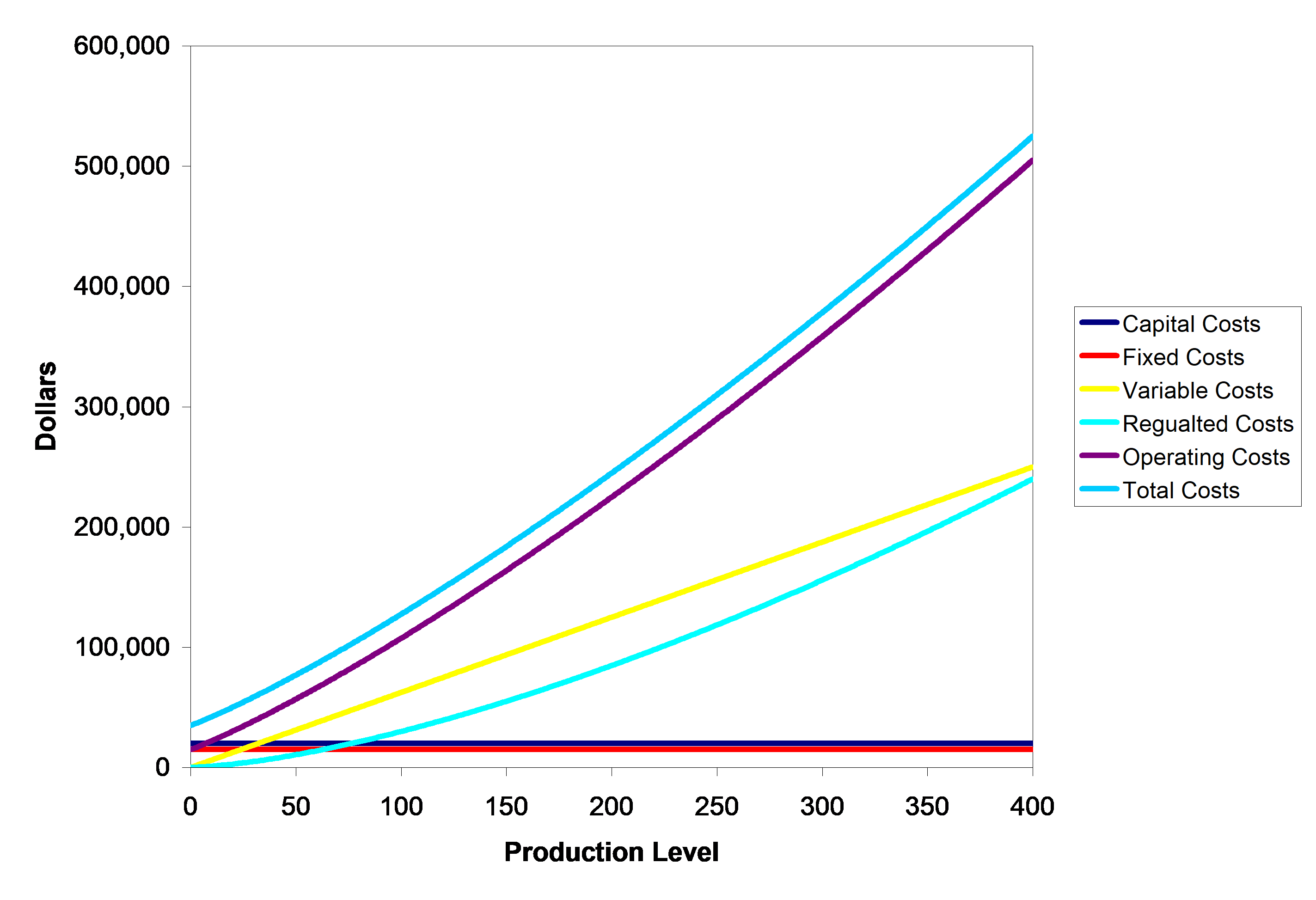
Figure 1 Capital, Fixed, Variable, Regulated, Operating, And Total Costs
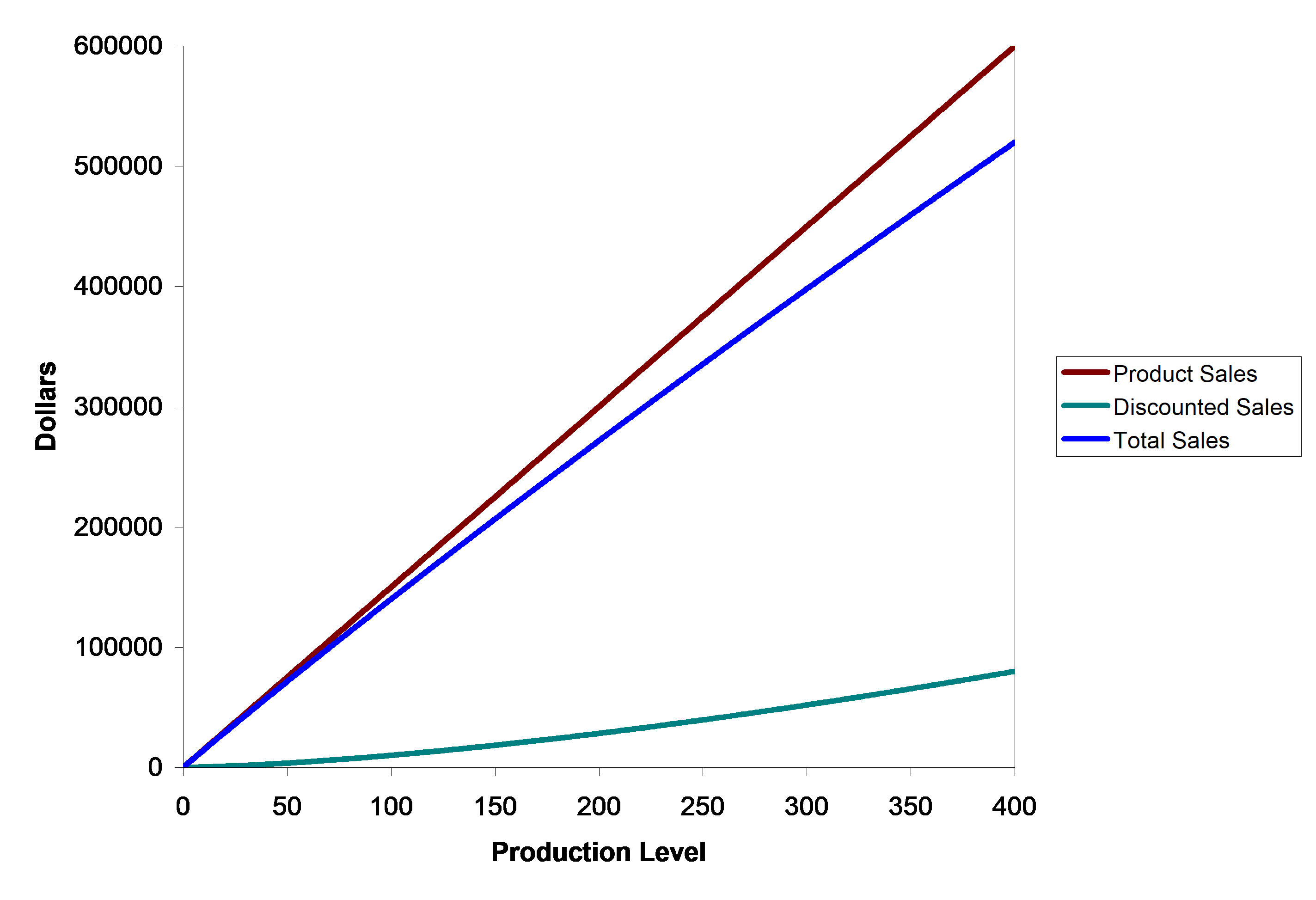
Figure 2 Product, Discounted, And Total Sales
All of the costs and sales revenue are shown next in Figure 3.
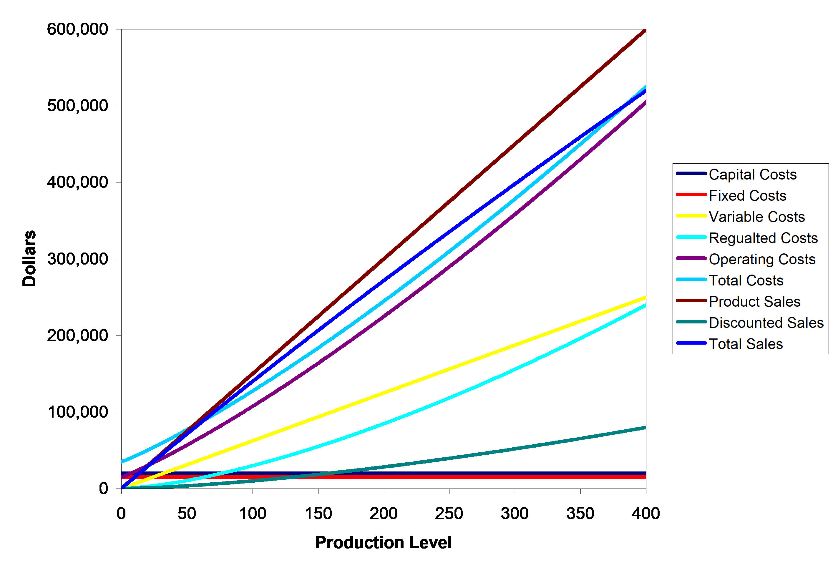
Figure 3 All of the Costs and Sales Revenue
At the break-even point there is no profit, so the capital cost plus the product cost equals the product sales (see Figure 4).
\[TC = TS\]
\[\$ 35,000 + \$ 625n + \$ 30n^{1.5} = \$ 1500n - \$ 10n^{1.5}\]
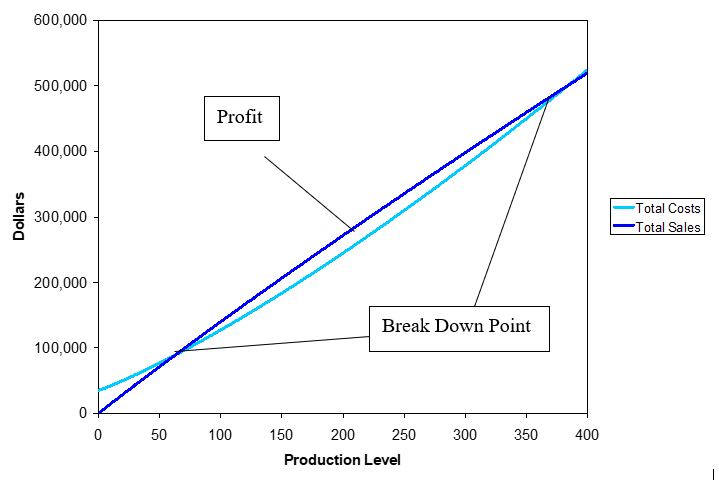
Figure 4 Break-Even Point and Profit Margin
Simplifying the previous equation yields the following nonlinear equation that needs to solved.
\[\$ 35,000 - \$ 875n + \$ 40n^{1.5} = 0\]
The value of \(n\) is the minimum number of computers that the shop will have to sell to make a profit. This is called the break-even point.
Questions
(1) Will some of the roots be complex for the above nonlinear equation?
(2) Using numerical techniques, we can solve this equation and any other equation of the form \(f(x) = 0\). Solve the above equation by all the methods you have learned assuming you want at least 3 significant digits to be correct in your answer.
(3) How can you use the knowledge of the problem to develop initial guess(es) for the numerical methods?
(4) Determine the production level that produces the most profit.
(5) Determine the second break-even point, after which a loss is realized.
(6) Reformulate the problem to determine the break-even point for the second year in business assuming that no capital costs are incurred.
Summary
A physical problem of finding how much cooling a shaft needs to be shrink fit into a hollow hub. The temperature to which the cooling needs to be done is modeled as a nonlinear equation.
Modeling
To make the fulcrum (Figure 1) of a bascule bridge, a long hollow steel shaft called the trunnion is shrink fit into a steel hub. The resulting steel trunnion-hub assembly is then shrink fit into the girder of the bridge.
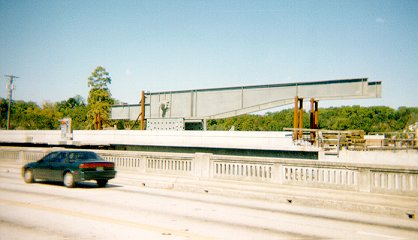
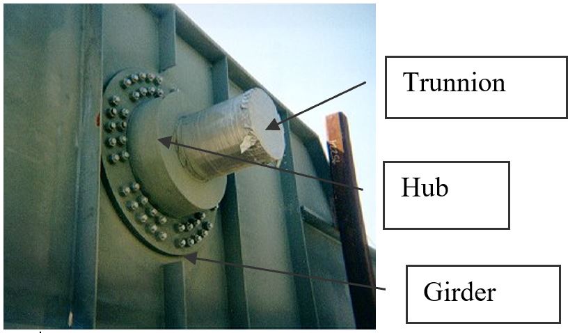
Figure 1 Trunnion-Hub-Girder (THG) assembly.
This is done by first immersing the trunnion in a cold medium such as dry-ice/alcohol mixture. After the trunnion reaches the steady state temperature of the cold medium, the trunnion outer diameter contracts. The trunnion is taken out of the medium and slid through the hole of the hub (Figure 2).
When the trunnion heats up, it expands and creates an interference fit with the hub. In 1995, on one of the bridges in Florida, this assembly procedure did not work as designed. Before the trunnion could be inserted fully into the hub, the trunnion got stuck. So a new trunnion and hub had to be ordered at a cost of $50,000. Coupled with construction delays, the total loss was more than a hundred thousand dollars.
Why did the trunnion get stuck? This was because the trunnion had not contracted enough to slide through the hole.
Now the same designer is working on making the fulcrum for another bascule bridge. Can you help him/her so that he does not make the same mistake?
For this new bridge, he needs to fit a hollow trunnion of the outside diameter \(12.363^{\prime\prime}\) in a hub of an inner diameter \(12.358^{\prime\prime}\). He plans to put the trunnion in dry-ice/alcohol mixture (temperature of the fluid - dry ice/alcohol mixture is \(- 108{^\circ}\text{F}\)) to contract the trunnion so that it can be slided through the hole of the hub. To slide the trunnion without sticking, he has also specified a diametrical clearance of at least \(0.01^{\prime\prime}\) between the trunnion and the hub. Assuming the room temperature is \(80{^\circ}\text{F}\), is immersing it in a dry-ice/alcohol mixture a correct decision? What temperature does he need to cool the trunnion to so that he gets the desired contraction?
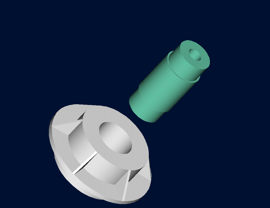
Figure 2 Trunnion slided through the hub after contracting
Looking at the designer’s record for the previous bridge (where the trunnion got stuck in the hub), it was found that they used the coefficient of linear thermal expansion at room temperature to calculate the contraction in the trunnion diameter. In that case, the reduction, \(\Delta D\) in the outer diameter of the trunnion is
\[\Delta D = D\alpha\Delta T\;\;\;\;\;\;\;\;\;\;\;\; (1)\]
where
\[D = \text{outer diameter of the trunnion,}\]
\[\alpha =\text{coefficient of linear thermal expansion at room temperature, and}\]
\[\Delta T = \text{change in temperature,}\]
Given
\[D = 12.363^{\prime\prime}\]
\[\alpha = 6.817 \times 10^{- 6}\text{in/in}{/}^{\circ}\text{F}\ \text{at}\ 80^{\circ}\text{F}\]
\[\begin{split} \Delta T &= T_{{fluid}} - T_{ {room}}\\ &= - 108 - 80\\ &= - 188^{\circ}\text{F} \end{split}\]
where
\[T_{ {fluid}}= \text{temperature of dry-ice/alcohol mixture}\]
\[T_{ {room}}= \text{room temperature}\]
the reduction in the trunnion outer diameter is given by
\[\begin{split} \Delta D &= (12.363)\left( 6.47 \times 10^{- 6} \right)\left( - 188 \right)\\ &= - 0.01504^{\prime\prime} \end{split}\]
So the trunnion is predicted to reduce in diameter by \(0.01504^{\prime\prime}\). But is this enough reduction in diameter? As per specifications, he needs the trunnion to contract by
\[\begin{split} &= \text{trunnion outside diameter} - \text{hub inner diameter} + \text{diametral clearance} \\ &=12.363^{\prime\prime} - 12.358^{\prime\prime} + 0.01^{\prime\prime}\\ &=0.015^{\prime\prime} \end{split}\]
So, according to his calculations, immersing the steel trunnion in dry-ice/alcohol mixture gives the desired contraction of \(0.015^{\prime\prime}\) as he is predicting a contraction of \(0.01504^{\prime\prime}\).
But as shown in Figure 3, the coefficient of linear thermal expansion of steel decreases with temperature and is not constant over the range of temperature the trunnion goes through. Hence the above formula (Equation 1) would overestimate the thermal contraction. This assumption is the mistake he made in the calculations for the earlier bridge.
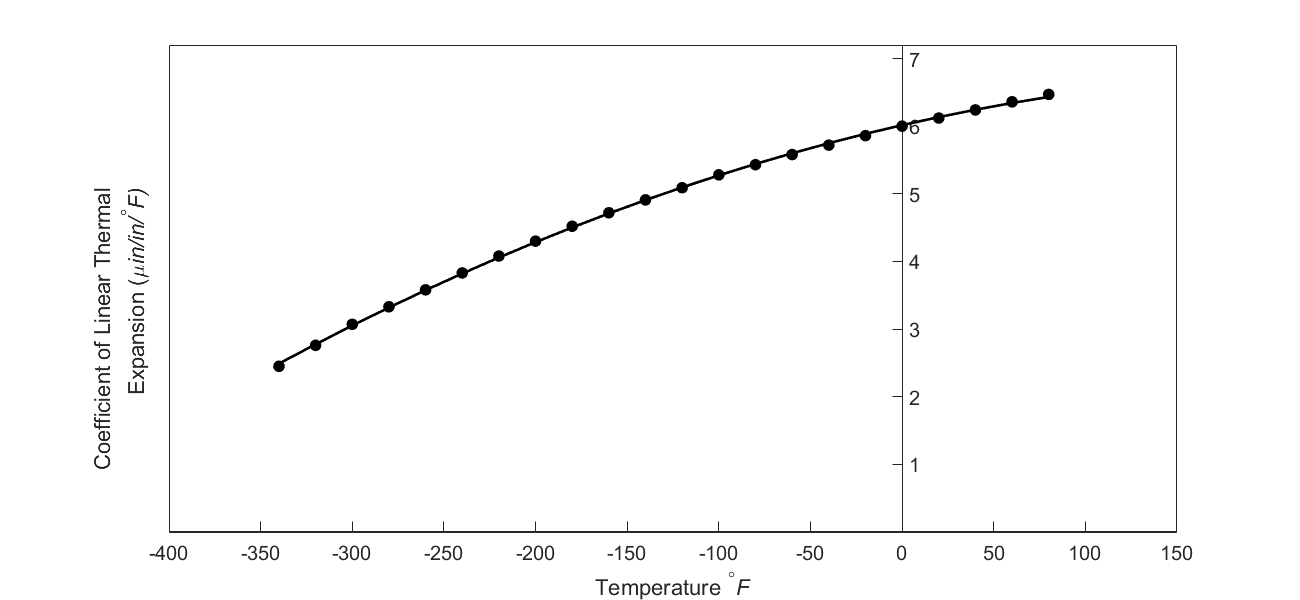
Figure 3 Varying coefficient of linear thermal expansion as a function of temperature for cast steel.
The contraction in the diameter for the trunnion for which the coefficient of linear thermal expansion varies as a function of temperature is given by
\[\Delta D = D\int_{T_{{room}}}^{T_{{fluid}}}{\alpha dT}\;\;\;\;\;\;\;\;\;\;\;\; (2)\]
Note that Equation (2) reduces to Equation (1) if the coefficient of linear thermal expansion is assumed to be constant. In Figure 3, the coefficient of linear thermal expansion of typical cast steel is approximated by a second-order polynomial as
\[\alpha = - 1.2278 \times 10^{- 11}T^{2} + 6.1946 \times 10^{- 9}T + 6.0150 \times 10^{- 6}\;\;\;\;\;\;\;\;\;\;\;\; (3)\]
Since the desired contraction is at least \(0.015^{\prime\prime}\), that is,
\[\Delta D = - 0.015^{\prime\prime},\;\;\;\;\;\;\;\;\;\;\;\; (4)\]
From Equations (2), (3), and (4),
\[- 0.015 = 12.363\int_{80}^{T_{{fluid}}}{\left( - 1.2278 \times 10^{- 11}T^{2} + 6.1946 \times 10^{- 9}T + 6.015 \times 10^{- 6} \right){dT}}\]
\[- 0.015 = 12.363\left\lbrack - 1.2278 \times 10^{- 11}\frac{T^{3}}{3} + 6.1946 \times 10^{- 9}\frac{T^{2}}{2} + 6.015 \times 10^{- 6}T \right\rbrack_{80}^{T_{{fluid}}}\]
\[{- 0.015 = 12.363( - 0.40927 \times 10^{- 11}T_{{fluid}}^{3} + 0.30973 \times 10^{- 8}T_{{fluid}}^{2} + 0.60150 \times 10^{- 5}T_{{fluid}} }{- 0.49893 \times 10^{- 3})}\]
\[f(T_{f}) = - 0.50598\ \times {1}{0}^{{-10}}T_{f}^{3} + 0.38292\ \times { 1}{0}^{{-7}}T_{f}^{2} + 0.74363 \times { 1}{0}^{{-4}}T_{f} + 0.88318\ \times {1}{0}^{{-2}} = 0\;\;\;\;\;\;\;\;\;\;\;\; (5)\]
One can solve this nonlinear equation to find the minimum fluid temperature needed to cool down the trunnion and get the desired contraction. Is cooling in dry-ice/alcohol mixture still your recommendation? You may be surprised that it would not be the correct decision to make.