Chapter 05.00: Physical Problem for Interpolation
Summary
The upward velocity of a rocket is given as a function of time at discrete data points. To find the velocity at a particular time requires interpolation.
Problem Statement
To find the altitude, velocity, and acceleration profile of a rocket, a velocity probe in the rocket (Figure 1) measures its velocity. Table 1 shows some typical values of the rocket velocity profile as a function of time.
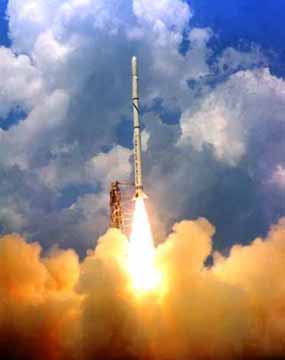
Figure 1 A rocket launched into space: Source: NASA Langley Research Center, Office of Education, edu.larc.nasa.gov/pstp/
To determine the velocity at a particular time, one needs to interpolate the velocity vs. time data. Although you may be familiar with linear interpolation, where you draw a straight line between two data points, you also want to know how accurate your estimate is. This forces you to use other interpolation functions such as quadratic and cubic polynomials.
Table 1. Velocity as a function of time
| \(t\ (\text{s})\) | \(v(t)\ (\text{m/s})\) |
|---|---|
| \(0\) | \(0\) |
| \(10\) | \(227.04\) |
| \(15\) | \(362.78\) |
| \(20\) | \(517.35\) |
| \(22.5\) | \(602.97\) |
| \(30\) | \(901.67\) |
Can you also find the distance covered by the rocket from one point of time to another? Can you find the acceleration of the rocket at a particular time?
Problem Statement
Well, I am from India and we are in the habit of drinking “afternoon tea.” The other day, my wife asked me to heat up some water in our kettle. I put 4 cups (you cannot have just 1 cup) of water in the kettle and put it on over our new flat-top burner.
“You are an engineer”, quipped my wife teasingly. “Can you estimate how long it would take for the water to boil and the kettle to make that whistling sound?” Yes, she clearly knows that whistling sound reminds me of all the horror movies that keep me awake at night.

Figure 1. A kettle of water on a flat burner.
Solution
A cup of water is about 200 ml in volume. So the total volume of water is about 800 ml. The burner for our flat top is rated at 1200 W. From first law of thermodynamics [1],
\[\Delta H + \Delta E_{p} + \Delta E_{k} = Q - W_{sh}\]
where
\[{\Delta H} = \text{change in internal energy,}\]
\[\Delta E_{p}= \text{change in potential energy,}\]
\[\Delta E_{k}= \text{change in kinetic energy,}\]
\[Q = \text{heat added to the system,}\]
\[W_{sh}= \text{work that is called shaft work.}\]
In this example
\[\Delta E_{p}=0,\]
\[\Delta E_{k}=0,\]
\[W_{sh}=0,\]
giving
\[\Delta H = Q.\]
Assuming no heat is lost as the kettle is assumed to be thermally insulated, the amount of heat needed is
\[\begin{split} Q &= \Delta H\\ &= mC_{p}{\Delta T} \end{split}\]
where
\[m = \text{mass of water (kg),}\]
\[C_{p}= \text{specific heat} \left( \frac{J}{{kg} -^{\circ}C} \right),\]
\[{\Delta T} = \text{change in temperature,}\]
and the values are given as
\[\begin{split} m &= 800{ml} \times \frac{{1kg}}{{1lit}}\\ &= 0.8kg \end{split}\]
\[C_{p}= 4814\frac{T}{{Kg} -^{\circ}K}\ \text{from (Reference [1] - Table 8.1)}\]
\[\begin{split} {\Delta T} &= 100^{\circ}C - 22^{\circ}C\\ &=78^{\circ}C \end{split}\]
Assuming that the room temperature is \(22^{\circ}C\) and the boiling temperature of water is \(100^{\circ}C\).
\[\begin{split} Q &= mC_{p}{\Delta T}\\ &= \left( 0.8 \right)\left( 4814 \right)\left( 78 \right)\\ &= 300394{J}. \end{split}\]
Since the wattage of the heater is 1200 W, the time it would take to boil is
\[\begin{split} &= \frac{300394}{1200}\\ &\cong 250\ s\\ &\cong 4 \text{min}\ 10\text{s} \end{split}\]
But, I do not see any interpolation here. One of the approximations made in the above formula is that the specific heat is constant over the temperature range of \(22^{\circ}C\) to \(100^{\circ}C\). But it is not a constant given in the Table 1.
Table 1. Specific heat of water as a function of temperature [2].
| Temperature | Specific heat |
|---|---|
| \(^{\circ}C\) | \(\frac{J}{{kg}{.}^{\circ}C}\) |
\(22\) \(42\) \(52\) \(82\) \(100\) |
\(4181\) \(4179\) \(4186\) \(4199\) \(4217\) |
One assumption one may make is to use the specific heat at the average temperature. In this case it is \(\displaystyle \frac{22 + 100}{2} = 61^{\circ}C\) .
So how do we find \(C_{p}\left( 61^{\circ}C \right)\)? We use interpolation to do that, that is, finding the value of a discrete function at a point that is not given to us. Using \(C_{p}\left( 61^{\circ}C \right)\) will give us a better estimate of how much time it would take to boil the water.
References
(1) Levenspiel, Octave, Understanding Engineering Thermo, Prentice Hall, New Jersey, 1996.
(2) Incropera, F.P. and DeWitt, D.P., Introduction to Heat Transfer, Wiley, 4th edition, 2001.
QUESTIONS
(1) Using the specific heat at the average temperature, how much is the difference in the estimated time for boiling the water.
(2) Use first, second and third order polynomial interpolation to estimate \(C_{p}\left( 61^{\circ}C \right)\) by all the methods (except spline) you learned in class. What is the absolute relative approximate error for each order of polynomial approximation? How many significant digits are at least correct in your solution.
(3) Just by looking at the data in Table 1, it may be clear that the calculated time using interpolation will not be very different from that found using the approximate specific heat. But in case of solids, it can be quite a different story. For example, to calculate heat required to raise the temperature of graphite from room temperature to \(800^{\circ}C\) for pyrolization, one needs to use proper specific heat data. Check yourself to see the difference between using specific heat at room temperature and specific heat at average temperature for the following problem. Find the heat required to raise the temperature of 1 kg of graphite from room temperature of \(22^{\circ}C\) to \(800^{\circ}C\), given the table of specific heat vs. temperature below.
Table 2 Specific heat of graphite as a function of temperature.
| Temperature | Specific heat |
|---|---|
| \(^{\circ} C\) | \(\frac{J}{{kg}.^{\circ}C}\) |
\(-73\) \(127\) \(327\) \(527\) \(727\) |
\(420\) \(1070\) \(1370\) \(1620\) \(1820\) |
Summary
Bass fishing never got so technical. Find how interpolation can help you to have a great catch and let you tell others a true fish story.
Problem Statement
This is a conversation between a former instructor (Autar) and civil engineering alumni named John Q. This is just what we heard!
Autar: “That is interesting! You are now a professional civil engineer and love to go bass fishing.”
John Q: “Actually, my civil engineering education is helping me in being a good bass fisherman!”
Autar: “How is that?”
John Q: “Well, if you know where the thermocline is in the lake, you can find a lot of bass there!”
Autar: “Glad I asked? Educate me.”
John Q: “Well, the water in a lake generally has three layers – epilimonon, thermocline and hypolimnion as shown in Figure 1 below. The thermocline layer is sandwiched between the epilimonon and the hypolimnion. The sun heats the water at the surface and this layer (epilimonon) of warm water floats over a layer (hypolimnion) of colder water, as the warm water is less dense then cold water. As days become hotter during the summer the layers become very distinct. Between these two layers of warm and cold water, you have a thin layer called the thermocline. Bass love the thermocline. So if you know where this thin layer of thermocline is, you can have a great catch.”
Autar: “But why do bass fish like the thermocline?”
John Q: “Well, the upper layer (epilimonon) has too much light for the bass to be calm, while the lower layer (hypolimnion) has too little oxygen. The thermocline is also ideal for algae growth. So, it is the place of choice for the bass. You will be wasting your time if you fish below the thermocline.”
Autar: “So how does one find where the thermocline is?”
John Q: “Well, you got electronic gadgets, such as depth finders, LCRs, and thermometers to do that. What some of these gadgets measure is the depth at which drastic change in temperature takes place? Just look at the data in Figure 2 taken in a lake in Pennsylvania. It shows the temperature data as a function of depth. You can see where it changes temperature suddenly. That is where the thermocline is.
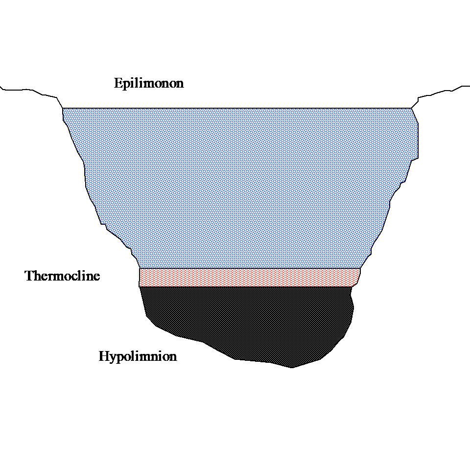
Figure 1 Three layers of lake stratification.
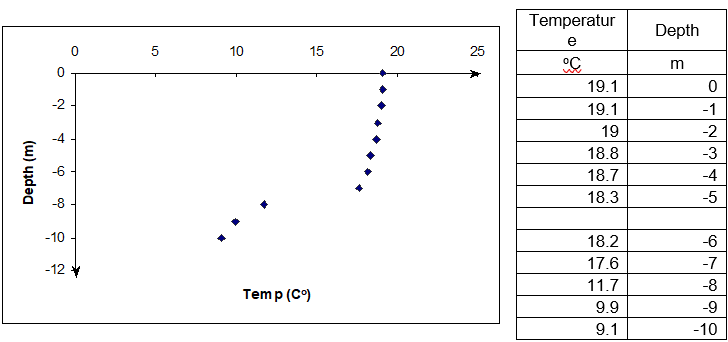
Figure 2 Temperature as a function of depth (Data courtesy of Ms. Bartlett - http://www.lehigh.edu/~infolios/becky/lakegraph.htm (last accessed January 2012).
Autar: “So what one can do is interpolate the temperature vs. depth data. The depth at which the thermocline occurs is the inflection point of the temperature-depth curve.”
John Q:”You are still in the habit of using jargon like inflection points. It still gives me beautiful dreams of Calculus II!”
Autar: “Yes, simply said, the inflection point is where the second derivative of temperature with respect to the depth becomes zero. That is \(\displaystyle\frac{d^{2}T}{dz^{2}} = 0\), where \(T\) is the temperature at depth \(z\). I think I am going to taking this problem to the classroom to teach my students about interpolation. Thanks to you.”
Summary
A robot arm path needs to be developed over several points on a flat plate. The path needs to be smooth to avoid sudden jerky motion and at the same time needs to be short.
Peter: “Dr. Kaw, I am taking a course in Manufacturing. We are solving the following problem. A robot arm with a rapid laser is used to do a quick quality check, such as hole radius, on six holes on a rectangular plate \(15^{\prime\prime} \times 10^{\prime\prime}\) at several points as shown in this table.
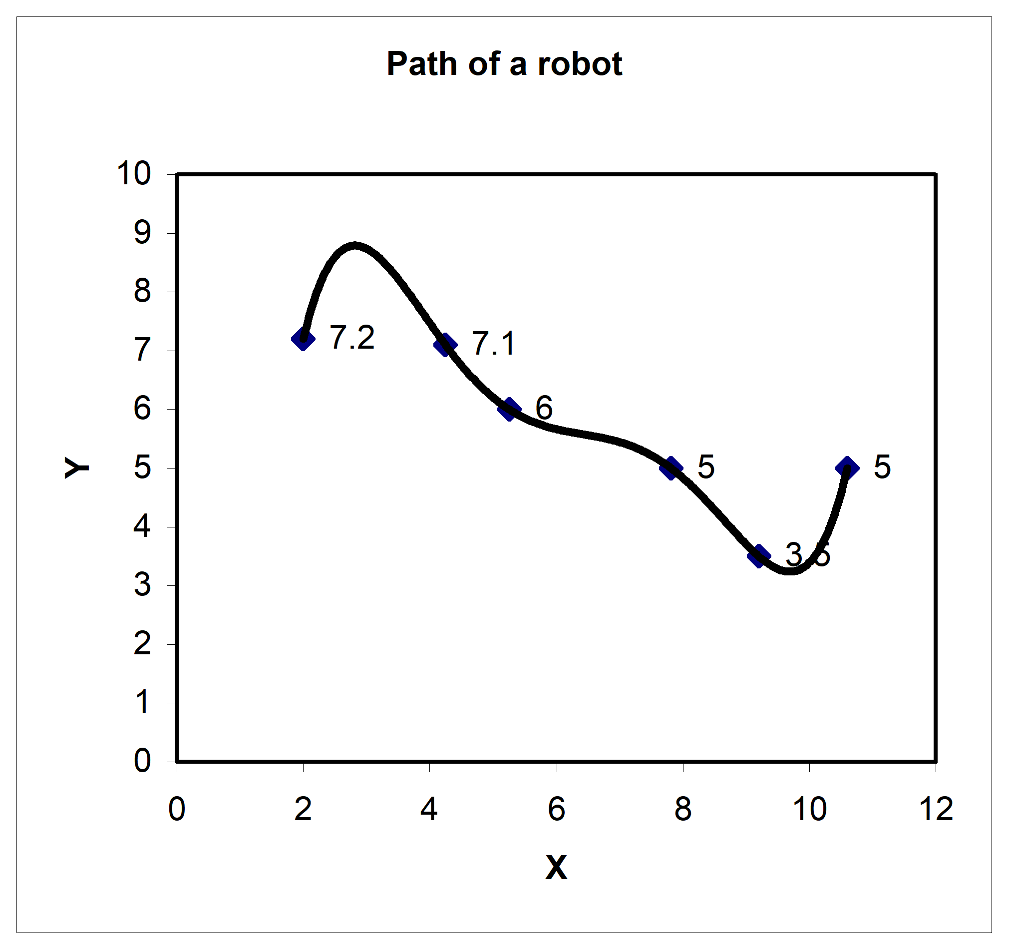
Figure 1. Path of a robot arm
Table 1. Coordinates of the points on the table
| X | Y |
|---|---|
| \(\mathbf{inches}\) | \(\mathbf{inches}\) |
| \(2.00\) | \(7.2\) |
| \(4.25\) | \(7.1\) |
| \(5.25\) | \(6.0\) |
| \(7.81\) | \(5.0\) |
| \(9.20\) | \(3.5\) |
| \(10.60\) | \(5.0\) |
I am using Excel to fit a fifth order polynomial through the 6 points. But, when I plot the polynomial, it is giving a long path!”
Kaw: “Why do you not just join the consecutive points by a straight line; just like the kids do at Pizza Hut with those ‘Connect the dots’ activities?”
Peter: “You are making me hungry and I wish it were that easy. The path of the robot going from one point to another needs to be smooth so as to avoid sharp jerks in the arm that can otherwise create premature wear and tear of the robot arm.”
Kaw: “As I recall, you took my course in Numerical Methods. What was that – one year ago?”
Peter: “Yes, your memory is sharp but my retention from that course – can we not talk about that!”
Kaw: “Come into my office. I wrote this program using Maple as you did. See this function, \(f(x) = 1/(1 + 25x^{2})\). I am choosing 7 points equidistantly between –1 and 1. Now look at the sixth order interpolating polynomial and the original function (See Figure 1). See the oscillations in the interpolating polynomial. In 1901, Runge [5] used this example function to show that higher order interpolation is a bad idea. A better alternative to getting a better representation of the curve is using splines. This is the solution to your problem as well. It will give you a smooth curve with less oscillations, and a shorter path. Try it!”
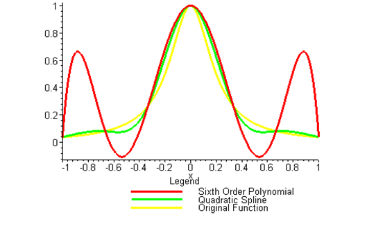
Figure 2 Runge’s function interpolated
Summary
Thermistors measure temperature based on the principle that resistance of thermistor material changes with temperature. Hence, a manufacturer supplies a resistance vs. temperature calibration curve. This curve is developed using interpolation.
Thermistors are temperature-measuring devices based on the principle that the thermistor material exhibits a change in electrical resistance with a change in temperature. By measuring the resistance of the thermistor material, one can then determine the temperature.
Thermistors are generally a piece of semiconductor made from metal oxides such as those of manganese, nickel, cobalt, etc. These pieces may be made into a bead, disk, wafer, etc depending on the application.
There are two types of thermistors – negative temperature coefficient (NTC) and positive temperature coefficient (PTC) thermistors. For NTCs, the resistance decreases with temperature, while for PTCs, the resistance increases with temperature. It is the NTCs that are generally used for temperature measurement.
Why would we want to use thermistors for measuring temperature as opposed to other choices such as thermocouples? It is because thermistors have high sensitivity giving more accuracy, a fast response to temperature changes for accuracy and quicker measurements, and relatively high resistance for decreasing the errors caused by the resistance of lead wires themselves.

Figure 1. A typical thermistor
But thermistors have a nonlinear output and are valued for a limited range. So, when a thermistor is manufactured, the manufacturer supplies a resistance vs. temperature curve. The curve generally used that gives an accurate representation is given by
\[\frac{1}{T} = a_{0} + a_{1}\ln(R) + a_{2}\left\{ \ln\left( R \right) \right\}^{2} + a_{3}\left\{ \ln\left( R \right) \right\}^{3} \ \ \ (1)\]
where
\[T\ \text{is temperature in Kelvin, and}\]
\[R\ \text{is resistance in ohms.}\]
\[a_{0},a_{1},a_{2},a_{3}\ \text{are constants of the calibration curve.}\]
Making change of variables
\[y = \frac{1}{T}, \text{ and}\]
\[x = \ln R,\]
we can change the calibration curve to a polynomial
\[y = a_{0} + a_{1}x + a_{2}x^{2} + a_{3}x^{3}.\]
So if one is able to find the constants of the above formula, one can then use the calibration curve to find the temperature.
Given below is the data of resistance vs. temperature for a thermistor. Can you find the calibration curve?
Table 1 Resistance vs. temperature data for calibration of a thermistor
| R | T |
|---|---|
| Ohm | \(^{\circ}C\) |
\(1101.0\) \(911.3\) \(636.0\) \(451.1\) |
\(25.113\) \(30.131\) \(40.120\) \(50.128\) |
References
[1] Betatherm sensors, http://www.betatherm.com
[2] Valvanao, J., “Measuring Temeparture Using Thermistors”, Curcuit Cellar Online, August 2000, http://www.circuitcellar.com/online
[3] Lavenuta, G., “Negative Temperature Coefficient Thermistors: Part 1: Characteristics, Materials, and Configurations”, http://www.globalspec.com/cornerstone/ref/negtemp.html
[4] Potter, D., “Measuring Temperature with Thermistors – a Tutorial”, National Instruments Application Note 065, http://www.seas.upenn.edu/courses/belab/ReferenceFiles/Thermisters/an065.pdf
[5] Steinhart, J.S. and Hart, S.R., 1968. “Calibration Curves for Thermistors,” Deep Sea Research 15:497.
[6] Sapoff, M. et al. 1982. “The Exactness of Fit of Resistance-Temperature Data of Thermistors with Third-Degree Polynomials,” Temperature, Its Measurement and Control in Science and Industry, Vol. 5, James F. Schooley, ed., American Institute of Physics, New York, NY:875.
[7] Siwek, W.R., et al. 1992. “A Precision Temperature Standard Based on the Exactness of Fit of Thermistor Resistance-Temperature Data Using Third Degree Polynomials,” Temperature, Its Measurement and Control in Science and Industry, Vol. 6, James F. Schooley, ed., American Institute of Physics, New York, NY:491-496.
Summary
To program a milling machine to make a cam profile, one needs to use interpolation to develop the path of the profile. The interpolation then requires a solution of simultaneous linear equations.
Problem Statement
An Industrial Engineer needs to program a Computer Numerical Control (CNC) milling machine to fabricate a cam profile that was designed by a Industrial Engineer to operate the intake valves in an internal combustion engine. The Mechanical Engineer’s task was to design a disk cam (rotating counterclockwise) to move a radial roller follower (in the vertical y-direction) as shown in Figure 1 below.
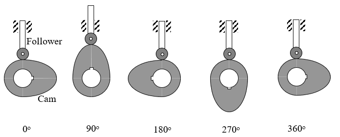
Figure 1 Motion of cam and follower.
Specifically, the cam is to move the follower as described in Table 1 below.
Table 1 Cam follower movement as a function of cam rotation.
| Cam rotation from X-axis | Follower movement in Y-direction |
|---|---|
| \(0^{\circ}\) | \(0.0\) |
| \(90^{\circ}\) | \(1.0\) |
| \(180^{\circ}\) | \(0.0\) |
| \(270^{\circ}\) | \(0.0\) |
| \(360^{\circ}\) | \(0.0\) |
Solution
The Mechanical Engineer has specified seven points along the profile of the cam (see Figure below) at \(30^{\circ}\) increments as shown in Figure 2 below.
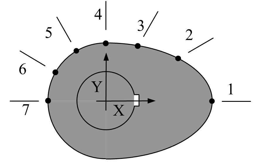
Figure 2 Schematic of cam profile
The geometry of the cam (i.e., coordinates of the seven points on the cam surface) are given in Table 2 below.
Table 2 Geometry of the cam.
| Point | Angle from X-axis | \(X\) | \(Y\) |
|---|---|---|---|
| 1 | \(-90^{\circ}\) | \(2.20\) | \(0.00\) |
| 2 | \(-60^{\circ}\) | \(1.28\) | \(0.88\) |
| 3 | \(-30^{\circ}\) | \(0.66\) | \(1.14\) |
| 4 | \(-0^{\circ}\) | \(0.00\) | \(1.20\) |
| 5 | \(30^{\circ}\) | \(-0.60\) | \(1.04\) |
| 6 | \(60^{\circ}\) | \(-1.04\) | \(0.60\) |
| 7 | \(90^{\circ}\) | \(-1.20\) | \(0.00\) |
The Industrial Engineer is responsible for fitting a smooth curve through the 7 points keeping in mind that the final curve must have a infinite slope at points 1 and 7, and zero slope at point 4.
Summary
Find the coefficient of linear thermal expansion of steel at a specific temperature to estimate whether a steel shaft will cool down enough to shrink fit into a hollow hub. The coefficient of linear thermal expansion is to be found by using interpolation from a given table of coefficient of linear thermal expansion of steel as a function of temperature.
Problem Statement
To make the fulcrum (Figure 1) of a bascule bridge, a long hollow steel shaft called the trunnion is shrink fit into a steel hub.
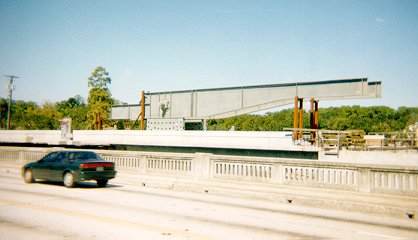
Figure 1 Trunnion-Hub-Girder (THG) assembly.
This is done by first immersing the trunnion in a cold medium such as a dry-ice/alcohol mixture. After the trunnion reaches a steady-state temperature, that is, the temperature of the cold medium, the trunnion outer diameter contracts, is taken out and slid through the hole of the hub (Figure 2).
Figure 2 Trunnion slid through the hub after contracting
When the trunnion heats up, it expands and creates an interference fit with the hub. In 1995, on one of the bridges in Florida, this assembly procedure did not work as designed. Before the trunnion could be inserted fully into the hub, the trunnion got stuck. So a new trunnion and hub had to be ordered worth $50,000. Coupled with construction delays, the total loss ran into more than a hundred thousand dollars.
Why did the trunnion get stuck? This was because the trunnion had not contracted enough to slide through the hole.
Now the same designer is working on making the fulcrum for another bascule bridge. Can you help him so that he does not make the same mistake?
For this new bridge, he needs to fit a hollow trunnion of an outside diameter \(12.363^{\prime\prime}\) in a hub of an inner diameter \(12.358^{\prime\prime}\). His plan is to put the trunnion in dry-ice/alcohol mixture (the temperature of dry ice/alcohol mixture is \(- 108{^\circ}\text{F}\)) to contract the trunnion so that it can be slid through the hole of the hub. To slide the trunnion without sticking, he has also specified a diametral clearance of at least \(0.01^{\prime\prime}\). Assume the room temperature is \(80{^\circ}\text{F}\), is immersing it in a dry-ice/alcohol mixture a correct decision?
Solution
Looking at the records of the designer for the previous bridge where the trunnion got stuck in the hub, it was found that he used the coefficient of linear thermal expansion at room temperature to calculate the contraction in the trunnion diameter. In that case, the reduction, \(\Delta D\) in the outer diameter of the trunnion is
\[\Delta D = D\alpha\Delta T\;\;\;\;\;\;\;\;\;\;\;\; (1)\]
where
\[D = \text{outer diameter of the trunnion,}\]
\[\alpha = \text{coefficient of linear thermal expansion at room temperature,}\]
\[\Delta T =\text{change in temperature.}\]
Given
\[D = 12.363^{\prime\prime}\]
\[\alpha = 6.817 \times 10^{- 6}\ \text{in/in/}{^\circ}\text{F}\ \text{at}\ 80{^\circ}\text{F}\]
\[\begin{split} \Delta T &= T_{\text{fluid}} - T_{\text{room}}\\ &= - 108 - 80\\ &= - 188{^\circ}\text{F} \end{split}\]
where
\[T_{{fluid}}= \text{temperature of dry-ice/alcohol mixture}\]
\[T_{{room}}= \text{room temperature}\]
the reduction in the trunnion outer diameter is given by
\[\begin{split} \Delta D &= 12.363 \times \left( 6.47 \times 10^{- 6} \right)\left( - 188 \right)\\ &= - 0.01504^{\prime\prime} \end{split}\]
So the trunnion is predicted to reduce in diameter by \(0.01504^{\prime\prime}\). But is this enough reduction in diameter? As per the specifications, he needs the trunnion to contract by
\[\begin{split} &= \text{trunnion outside diameter} - \text{hub inner diameter} + \text{diametric clearance}\\ &=12.363^{\prime\prime} - 12.358^{\prime\prime} + 0.01^{\prime\prime}\\ &=0.015^{\prime\prime} \end{split}\]
So, according to his calculations, it is enough to put the steel trunnion in a dry-ice/alcohol mixture to get the desired contraction of \(0.015^{\prime\prime}\) as he is predicting a contraction of \(0.01504^{\prime\prime}\).
But as shown in the graph below, the coefficient of linear thermal expansion of steel decreases with temperature and is not constant over the range of temperature the trunnion goes through. Hence the above formula (Equation 1) would overestimate the thermal contraction. This assumption is the mistake he made in the calculations for the earlier bridge.
Figure 3 Varying coefficient of linear thermal expansion as a function of temperature for cast steel.
To get a better estimate of the contraction in the diameter, we can use the coefficient of linear thermal expansion value at the average temperature. The average temperature would be
\[\begin{split} T_{{avg}} &= \frac{- 108 + 80}{2}\\ &= -14^{\circ}\text{F} \end{split}\;\;\;\;\;\;\;\;\;\;\;\; (2)\]
Now given the table of coefficient of linear thermal expansion as a function of temperature as given below, we can use polynomial interpolation to find the coefficient of linear thermal expansion at the average temperature of \(- 14^{\circ}F\) and find the contraction using Equation (1).
Table 1 Coefficient of linear thermal expansion vs. temperature
| Temperature (\(^\circ \text{F}\)) | coefficient of linear thermal expansion (\({\mu}\text{in/in}{/}^{\circ}\text{F}\)) |
|---|---|
| \(80\) | \(6.47\) |
| \(60\) | \(6.36\) |
| \(40\) | \(6.24\) |
| \(20\) | \(6.12\) |
| \(0\) | \(6.00\) |
| \(-20\) | \(5.86\) |
| \(-40\) | \(5.72\) |
| \(-60\) | \(5.58\) |
| \(-80\) | \(5.43\) |
| \(-100\) | \(5.28\) |
| \(-120\) | \(5.09\) |
| \(-140\) | \(4.91\) |
| \(-160\) | \(4.72\) |
| \(-180\) | \(4.52\) |
| \(-200\) | \(4.30\) |
| \(-220\) | \(4.08\) |
| \(-240\) | \(3.83\) |
| \(-260\) | \(3.58\) |
| \(-280\) | \(3.33\) |
| \(-300\) | \(3.07\) |
| \(-320\) | \(2.76\) |
| \(-340\) | \(2.45\) |