Chapter 06.05: Adequacy of Linear Regression Models
Learning Objectives
After successful completion of this lesson, you should be able to:
1) find why adequacy of a linear regression model is critical,
2) answer the two questions that need to be considered for a linear regression model to be adequate.
Introduction
In the application of regression models, one objective is to obtain an equation \(y = f(x)\) that best describes the \(n\) response data points \((x_{1},y_{1}),(x_{2},y_{2}),\ldots\ldots,(x_{n},y_{n})\). Consequently, we are faced with answering two basic questions.
1) Does the model \(y = f(x)\) describe the data adequately, that is, is there an adequate fit?
2) How well does the model predict the response variable (predictability)?
To answer these questions, we limit our discussion to straight-line models as nonlinear models require a different approach. Some authors claim that nonlinear model parameters are not unbiased.
For our discussion, we take example data to go through the process of model evaluation. Given below is the data for the coefficient of thermal expansion vs. temperature for steel.
Table 1. Values of the coefficient of thermal expansion vs. temperature.
| \(T\ (^{\circ}\text{F})\) | \(\alpha\ (\mu \text{in/in}{/}^{\circ}\text{F})\) |
|---|---|
\(-340\) \(-260\) \(-180\) \(-100\) \(-20\) \(60\) |
\(2.45\) \(3.58\) \(4.52\) \(5.28\) \(5.86\) \(6.36\) |
We assume a linear relationship between the coefficient of thermal expansion and temperature data as
\[\alpha(T) = a_{0} + a_{1}T\;\;\;\;\;\;\;\;\;\;\;\; (1)\]
Following the procedure for conducting linear regression as given in a previous lesson, we get
\[\alpha(T) = 6.0325 + 0.0096964T\;\;\;\;\;\;\;\;\;\;\;\; (2)\]
The adequacy of a linear regression model can be determined through four checks.
1) Check if the data and corresponding regression line look visually acceptable.
2) Check how many scaled residuals are in the \([-2,2]\) range.
3) Check the coefficient of determination.
4) Check the assumption of the inherent randomness of the residuals.
The procedure to make these checks and the criteria for acceptability are discussed in the next lesson.
Learning Objectives
After successful completion of this lesson, you should be able to:
1) Make the first check of the adequacy of the regression model by plotting the data and the linear regression model.
2) Calculate a standard estimate of the error.
3) Calculate scaled residuals.
4) Make the second check of the adequacy of the linear regression model by calculating how many scaled residuals are in the [-2,2] bracket.
5) Calculate the coefficient of determination.
6) Calculate correlation coefficient.
7) Make the third check of the adequacy of the linear regression model by calculating how close the coefficient of determination is to 1.
8) Make the fourth check of the adequacy of the linear regression model by calculating if it meets the assumptions of random errors.
Check 1. Plot the data and the regression model.
In this check, we visually check the plot of the data and the regression model. As an example, given below is the data for the coefficient of thermal expansion vs. temperature for steel.
Table 1. Values of the coefficient of thermal expansion vs. temperature.
| \(T(^{\circ}\text{F})\) | \(\alpha\ (\mu \text{in/in}{/}^{\circ}\text{F})\) |
|---|---|
\(-340\) \(-260\) \(-180\) \(-100\) \(-20\) \(60\) |
\(2.45\) \(3.58\) \(4.52\) \(5.28\) \(5.86\) \(6.36\) |
We assume a linear relationship between the coefficient of thermal expansion and temperature data as
\[\alpha(T) = a_{0} + a_{1}T\;\;\;\;\;\;\;\;\;\;\;\; (1)\]
Following the procedure for conducting linear regression as given in the earlier lessons, we get
\[\alpha(T) = 6.0325 + 0.0096964T\;\;\;\;\;\;\;\;\;\;\;\; (2)\]
Figure 1 shows the data and the regression model.
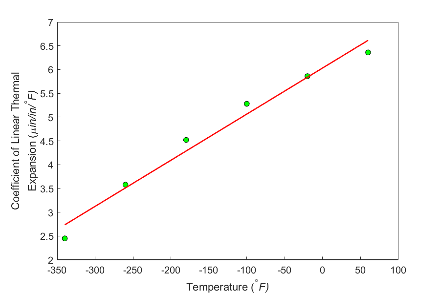
Figure 1. Plot of the coefficient of thermal expansion vs. temperature data points and regression line.
So what is the check? From a visual check, the regression line and the data are close to each other, and it looks like the model explains the data adequately.
Check 2. Is the standard estimate of error within bounds?
Denoted by \(s_{y/x}\) for y vs. x data, the standard error of estimate is used in the criterion to check the adequacy of a linear regression model.
For \(y\) vs. \(x\) data with \(n\) data points, the standard error of estimate \(\displaystyle s_{y/x}\) is defined as
\[s_{y/x} = \sqrt{\frac{S_{r}}{n - 2}}\;\;\;\;\;\;\;\;\;\;\;\; (3)\]
where
\[S_{r} = \sum_{i = 1}^{n}{(y_{i} - a_{0} - a_{1}x_{i})^{2}}\;\;\;\;\;\;\;\;\;\;\;\; (4)\]
Take the same example for data given in Table 1. The residuals for the data are given in Table 2.
Table 2 Residuals for data.
| \(T_{i}\) | \(\alpha_{i}\) | \(a_0 + a_{1}T_{i}\) | \(\alpha_{i} - a_{0} - a_{1}T_{i}\) |
|---|---|---|---|
\(-340\) \(-260\) \(-180\) \(-100\) \(-20\) \(60\) |
\(2.45\) \(3.58\) \(4.52\) \(5.28\) \(5.86\) \(6.36\) |
\(2.7357\) \(3.5114\) \(4.2871\) \(5.0629\) \(5.8386\) \(6.6143\) |
\(-0.28571\) \(0.068571\) \(0.23286\) \(0.21714\) \(0.021429\) \(-0.25429\) |
Calculate the sum of the square of residuals as
\[\begin{split} S_{r} &= ( - 0.28571)^{2} + (0.068571)^{2} + (0.23286)^{2}\\ &\ \ \ \ \ +(0.21714)^2+(0.021429)^2+(-0.25429)^2\\ &= 0.25283\end{split}\]
The standard error of estimate as given by Equation (3) is
\[\begin{split} \displaystyle s_{\alpha/T} &= \sqrt{\frac{S_{r}}{n - 2}}\\ &= \sqrt{\frac{0.25283}{6 - 2}}\\ &= 0.25141 \end{split}\]
The units of \(s_{\alpha/T}\) are the same as the units of \(\alpha\).
How is the value of the standard error of estimate interpreted? We may say that, on average, the absolute difference between the observed and predicted values is \(s_{\alpha/T}\), that is, \(0.25141\ \mu \text{in/in}{/}^{\circ}\text{F}\). We can also look at the value of \(s_{\alpha/T}\) as follows. The observed \(\alpha\) values are between \(\pm 2s_{\alpha/T}\) of the predicted value (see Figure 1). This would lead us to believe that the value of \(\alpha\) in the example is expected to be accurate within \(\pm 2s_{\alpha/T}\)=\(\pm 2 \times 0.25141\)=\(\pm 0.50282\ \mu \text{in/in}{/}^{\circ}\text{F}\).
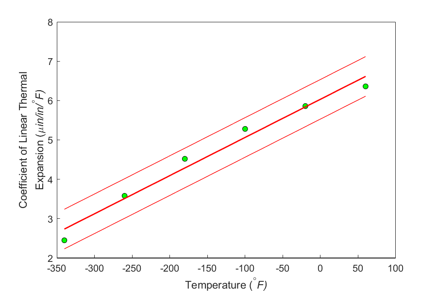
Figure 2. Plotting the linear regression line and showing the regression standard error.
So what is the check? Check if \(95\%\) of the observed \(\alpha\) values are between \(\pm 2s_{\alpha/T}\) of the predicted value. Since it would be impractical to visually make this observation for a large data set, one needs to do so programmatically. Simply calculate the scaled residual for each data pair as given by dividing the residual by the standard error of estimate.
\[\text{Scaled residual}= \displaystyle \frac{\alpha_{i} - a_{0} - a_{1}T_{i}}{s_{\alpha/T}}\;\;\;\;\;\;\;\;\;\;\;\; (5)\]
and check if \(95\%\) of the scaled residuals are in \([-2, 2]\) domain.
For this example,
\[s_{\alpha/T} = 0.25141\]
and the scaled residuals are shown in Table 3.
Table 3. Residuals and scaled residuals for data.
| \(T_{i}\) | \(\alpha_{i}\) | \(\alpha_{i} - a_{0} - a_{1}T_{i}\) | \(\text{Scaled Residuals}\) |
|---|---|---|---|
\(-340\) \(-260\) \(-180\) \(-100\) \(-20\) \(60\) |
\(2.45\) \(3.58\) \(4.52\) \(5.28\) \(5.86\) \(6.36\) |
\(-0.28571\) \(0.068571\) \(0.23286\) \(0.21714\) \(0.021429\) \(-0.25429\) |
\(-1.1364\) \(0.27275\) \(0.92622\) \(0.86369\) \(0.085235\) \(-1.0115\) |
All the scaled residuals are in the \([-2,2]\) domain, and hence \(95\%\) or more of the scaled residuals are in the \([-2,2]\) domain. It looks like the model explains the data adequately.
Check 3. How close is the coefficient of determination to one?
Denoted by \(r^{2}\), the coefficient of determination is used in another criterion for checking the adequacy of the linear regression model.
To find the formula for the coefficient of determination, let us start examining some measures of discrepancies between the whole data and some key central tendency. Look at the two equations given below.
\[S_{r} = \sum_{i = 1}^{n}\left( \alpha_{i} - a_{0} - a_{1}T_{i} \right)^{2}\;\;\;\;\;\;\;\;\;\;\;\; (6)\]
\[S_{t} = \sum_{i = 1}^{n}\left( \alpha_{i} - \bar{\alpha} \right)^{2}\;\;\;\;\;\;\;\;\;\;\;\; (7)\]
where
\[\bar{\alpha} = \frac{\displaystyle \sum_{i = 1}^{n}\alpha_{i}}{n}\]
Equation (6) is the spread of the data from the regression model (called the sum of the squares of the residuals, \(S_{r}\)) and Equation (7) is the spread of the data from the average (called the total sum of squares, \(S_{t}\)).
For the example data
\[\begin{split} \bar{\alpha} &= \frac{\displaystyle\sum_{i = 1}^{6}\alpha_{i}}{6}\\ &= \frac{2.45 + 3.58 + 4.52 + 5.28 + 5.86 + 6.36}{6}\\ &= 4.6750\ {\mu in}/{in}/{^\circ}F \end{split}\]
Table 4 shows the difference between observed values and the average.
Table 4. Difference between observed values and the average.
| \(T_{i}\) | \(\alpha_{i}\) | \(\alpha_{i} - \bar{\alpha}\) |
|---|---|---|
\(-340\) \(-260\) \(-180\) \(-100\) \(-20\) \(60\) |
\(2.45\) \(3.58\) \(4.52\) \(5.28\) \(5.86\) \(6.36\) |
\(-2.2250\) \(-1.0950\) \(-0.15500\) \(0.60500\) \(1.1850\) \(1.6850\) |
Using Equation (7), the total sum of squares, \(S_{t}\) (see column 3 of Table 5), is
\[\begin{split} S_{t} &= \sum_{i = 1}^{n}\left( \alpha_{i} - \bar{\alpha} \right)^{2}\\ &=(-2.2250)^2+(-1.0950)^2+(-0.15500)^2 + (0.60500)^{2} + (1.1850)^{2} + (1.6850)^{2}\\ &= 10.783\end{split}\]
Table 5 shows the residuals of the data.
Table 5. Residuals for data.
| \(T_{i}\) | \(\alpha_{i}\) | \(a_{0} + a_{1}T_{i}\) | \(\alpha_{i} - a_{0} - a_{1}T_{i}\) |
|---|---|---|---|
\(-340\) \(-260\) \(-180\) \(-100\) \(-20\) \(60\) |
\(2.45\) \(3.58\) \(4.52\) \(5.28\) \(5.86\) \(6.36\) |
\(2.7357\) \(3.5114\) \(4.2871\) \(5.0629\) \(5.8386\) \(6.6143\) |
\(-0.28571\) \(0.068571\) \(0.23286\) \(0.21714\) \(0.021429\) \(-0.25429\) |
Using Equation (6), the sum of the square of residuals (see Column 4 of Table 6) is
\[\begin{split} S_{r} &= ( - 0.28571)^{2} + (0.068571)^{2} + (0.23286)^{2} + (0.21714)^{2}\\ & \ \ \ \ \ + (0.021429)^{2} + ( - 0.25429)^{2}\\ &= 0.25283\end{split}\]
What inferences can we make from Equations (6) and (7)?
Equation (7) measures the discrepancy between the data and the average. Recall that the average of the data is a single value that measures the central tendency of the whole data. Equation (7) contrasts with Equation (6) as Equation (6) uses the vertical distance of the point from the regression line (another measure of central tendency) to measure the tendency from the straight line.
The objective of least-squares method is to obtain a compact equation that best describes all the data points. The mean can also be used to describe all the data points. The magnitude of the sum of squares of deviation from the mean or from the least-squares line is, therefore, a good indicator of how well the mean or least-squares characterizes the whole data, respectively. We can liken the sum of squares deviation around the mean \(S_{t}\) as the error or variability in the dependent variable\(\ y\) without considering the independent variable \(x\), while \(S_{r}\) as the sum of squares deviation around the least square regression line or variability in \(y\) remaining after the variability with\(\ x\) has been considered.
The difference between these two parameters \((S_{t} - S_{r})\) measures the error due to describing or characterizing the data. However, \((S_{t} - S_{r})\) value by itself is not a good criterion to use. Just see for yourself in the example how this difference would be perceived differently for the example data if we changed the units of the predicted variable \(\alpha\) from \((\mu \text{in/in/}{^\circ}\text{F})\) to \((\text{in/in/}{^\circ}\text{F})\). The value of \((S_{t} - S_{r})\) is \(10.53017\) when units of \((\mu i\text{in/in/}{^\circ}\text{F})\) are used, and \(10.53017 \times 10^{- 12}\) when units of \((\text{in/in/}{^\circ}\text{F})\) are used.
A relative comparison of this difference \((S_{t} - S_{r})\) to \(S_{t}\) is a better-normalized indicator and is defined as the coefficient of determination \(r^{2}\), where
\[r^{2} = \frac{S_{t} - S_{r}}{S_{t}}\;\;\;\;\;\;\;\;\;\;\;\; (8)\]
For the example
\[\begin{split} r^{2} &= \frac{10.783 - 0.25283}{10.783}\\ &= 0.97655 \end{split}\]
The limits of the values of \(r^{2}\) are between \(0\) and \(1\). What do these limiting values of \(r^{2}\) mean? If \(r^{2} = 0\), then \(S_{t} = S_{r}\), which means that regressing the data to a straight line does nothing to explain the data any further. If \(r^{2} = 1\), then \(S_{r} = 0\), which means that the straight line passes through all the data points and is a perfect fit.
So what is the check? Based on the value obtained above for \(r^{2} = 0.97655\), we can claim that \(97.7\%\) of the original uncertainty in the value of \(\alpha\) can be explained by the straight-line regression model
\[\alpha(T) = 6.0325 + 0.0096964T.\]
This high value of \(r^{2}\), close to \(1\), means that the linear regression model is adequate based on this criterion.
Correlation Coefficient: The square root of the coefficient of determination \(r^{2}\) is called the correlation coefficient, r. It can vary from \(- 1\) to \(1\) and represents the strength of the association between the predicted (dependent) and predictor (independent) variables. The sign of the correlation coefficient is the same as the sign of the slope of the linear regression line. As a simple rule of thumb, the strength of the correlation (Table 6) is interpreted by the absolute value of the correlation coefficient.
Table 6. Strength of correlation
| \(|r|\) | \(\text{Correlation Interpretation}\) |
|---|---|
| \(0.80\ \text{to}\ 1.00\) | \(\text{Very Strong}\) |
| \(0.60\ \text{to}\ 0.79\) | \(\text{Strong}\) |
| \(0.40\ \text{to}\ 0.59\) | \(\text{Moderate}\) |
| \(0.20\ \text{to}\ 0.39\) | \(\text{Low}\) |
| \(0.00\ \text{to}\ 0.19\) | \(\text{Little or none}\) |
For the example
\[\begin{split} r &= \sqrt{0.97655}\\ &= + 0.98820 \end{split}\]
The value is positive because the slope of the linear regression curve is positive. The high value of the correlation coefficient can be interpreted as a very strong correlation between the predicted variable \(\alpha\) and the predictor variable T.
Check 4. Find if the model meets the assumptions of random errors.
These assumptions include 1) that the residuals are negative as well as positive to give a mean of zero, 2) the variation of the residuals as a function of the independent variable is random, 3) the residuals follow a normal distribution, and 4) that there is no auto-correlation between the data points.
To illustrate this better, we have an extended data set for the example that we took. Instead of 6 data points, this set has 22 data points (Table 7). Drawing conclusions from small or large data sets for checking the assumption of random error is not recommended.
Table 7. Instantaneous thermal expansion coefficient as a function of temperature.
| Temperature | Instantaneous Thermal Expansion |
|---|---|
| \(^\circ \text{F}\) | \(\mu \text{in/in/}^\circ \text{F}\) |
| \(80\) | \(6.47\) |
| \(60\) | \(6.36\) |
| \(40\) | \(6.24\) |
| \(20\) | \(6.12\) |
| \(0\) | \(6.00\) |
| \(-20\) | \(5.86\) |
| \(-40\) | \(5.72\) |
| \(-60\) | \(5.58\) |
| \(-80\) | \(5.43\) |
| \(-100\) | \(5.28\) |
| \(-120\) | \(5.09\) |
| \(-140\) | \(4.91\) |
| \(-160\) | \(4.72\) |
| \(-180\) | \(4.52\) |
| \(-200\) | \(4.30\) |
| \(-220\) | \(4.08\) |
| \(-240\) | \(3.83\) |
| \(-260\) | \(3.58\) |
| \(-280\) | \(3.33\) |
| \(-300\) | \(3.07\) |
| \(-320\) | \(2.76\) |
| \(-340\) | \(2.45\) |
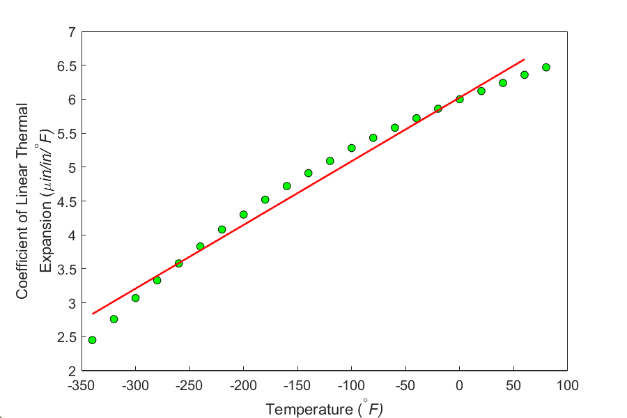
Figure 3. Plot of thermal expansion coefficient vs. temperature data points and regression line for more data points.
Regressing the data from Table 7 to the straight-line regression line
\[\alpha(T)=a_0+a_1T\]
and following the procedure for conducting linear regression as given in Chapter 06.03, we get (Figure 3)
\[\alpha=6.0248+0.0093868T\;\;\;\;\;\;\;\;\;\;\;\; (9)\]
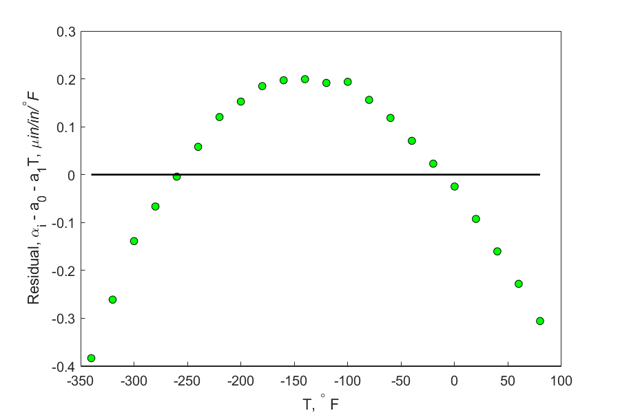
Figure 4. Plot of residuals.
Figure 4 shows the residuals for the example as a function of temperature. Although the residuals seem to average to zero, but within a range, they do not exhibit this zero mean. For an initial value of \(T\), the averages are below zero. For the middle values of \(T\), the averages are above zero, and again for the final values of \(T\), the averages are below zero. This non-random variation may be considered a violation of the model assumption.
Figure 4 also shows that the residuals for the example are following a nonlinear variance which is a clear violation of the model assumption of constant variance.
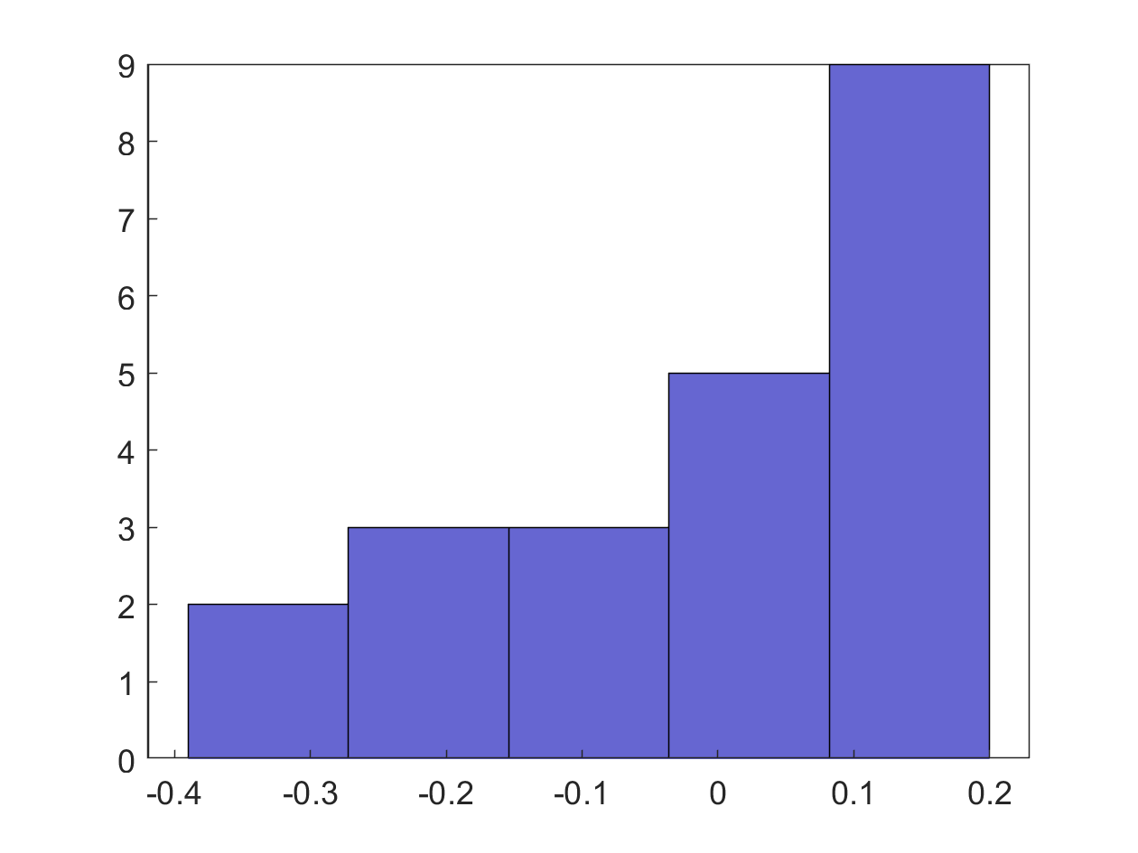
Figure 5. Histogram of residuals.
Figure 5 shows the histogram of the residuals. Clearly, the histogram is not showing a normal distribution and hence violates the model assumption of normality.
To check that there is no autocorrelation between observed values, the following rule of thumb can be used. If \(n\) is the number of data points, and \(q\) is the number of times the sign of the residual changes, then if
\[\frac{(n-1)}{2}-\sqrt{n-1}\le\ q\le\frac{n-1}{2}+\sqrt{n-1}\;\;\;\;\;\;\;\;\;\;\;\; (10)\]
you most likely do not have an autocorrelation. For the example, \(n=22\), then
\[\frac{(22-1)}{2}-\sqrt{22-1}\le\ q\le\frac{22-1}{2}+\sqrt{22-1}\]
\[5.9174\le\ q\le15.083\]
is not satisfied as \(q=2\). So this model assumption is violated.
Learning Objectives
After successful completion of this lesson, you should be able to:
1) enumerate abuses of regression
2) give examples related to abuses of regression.
Introduction
There are three common cases of abuse of regression analysis. They are the following.
1) Extrapolation
2) Generalization
3) Misidentification
Extrapolation
If you were dealing in the stock market or even interested in it, then you might remember the stock market crash of March 2000. During 1997-1999, investors thought they would double their money every year. They started buying fancy cars and houses on credit and living a high life. Little did they know that the whole market was hyped on speculation and little economic sense. The Enron and MCI financial fiascos soon followed.
Let us look if we could have safely extrapolated the NASDAQ index from past years. Below is the table of NASDAQ index, \(S\), as a function of the end of year number, \(t\) (Year 1 is the end of the year 1994, and Year 6 is the end of the year 1999).
Table 1 NASDAQ index as a function of year number.
| Year Number, t | NASDAQ Index {S} |
|---|---|
| \(1\ (1994)\) | \(752\) |
| \(2\ (1995)\) | \(1052\) |
| \(3\ (1996)\) | \(1291\) |
| \(4\ (1997)\) | \(1570\) |
| \(5\ (1998)\) | \(2193\) |
| \(6\ (1999)\) | \(4069\) |
Note: NASDAQ (National Association of Securities Dealers Automated Quotations) index is a composite index based on the stock market value of 3,000 companies. The NASDAQ index began on February 5, 1971, with a base value of 100. Twenty years later, in 1995, the NASDAQ index crossed the 1000 mark. It rose as high as 5132 on March 10, 2000, and currently is at a value of 13829 (April 8, 2021).
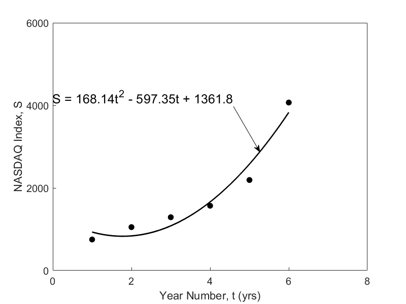
Figure 1 The regression line of the NASDAQ Index as a function of year number.
A relationship \(S = a_{0} + a_{1}t + a_{2}t^{2}\) between the NASDAQ index, \(S\), and the year number, \(t\), is developed using least square regression and is found to be \(S = 168.14t^{2} - 597.37t + 1361.8\). The data and the regression line are shown in Figure 1. The data is given only for Years 1 through 6, and it is desired to calculate the value for \(t > 6,\) and that is extrapolation outside the model data. The error inherent in this model is shown in Table 2 and Figure 2. Look at the Year 7 and 8 that were not included in the data – the error between the predicted and actual values is \(119\%\) and \(277\%\), respectively.
Table 2 NASDAQ index as a function of year number.
Year Number (\(\mathbf{t}\)) |
NASDAQ Index (\(\mathbf{S}\)) |
Predicted Index |
Absolute Relative True Error (%) |
|---|---|---|---|
| \(1\ (1994)\) | \(752\) | \(933\) | \(24\) |
| \(2\ (1995)\) | \(1052\) | \(840\) | \(20\) |
| \(3\ (1996)\) | \(1291\) | \(1083\) | \(16\) |
| \(4\ (1997)\) | \(1570\) | \(1663\) | \(6\) |
| \(5\ (1998)\) | \(2193\) | \(2579\) | \(18\) |
| \(6\ (1999)\) | \(4069\) | \(3831\) | \(6\) |
| \(7\ (2000)\) | \(2471\) | \(5419\) | \(119\) |
| \(8\ (2001)\) | \(1951\) | \(7344\) | \(276\) |
This illustration is not exaggerated, and it is important that careful use of any given model equation is always employed. At all times, it is imperative to infer the domain of independent variables for which a given equation is valid.
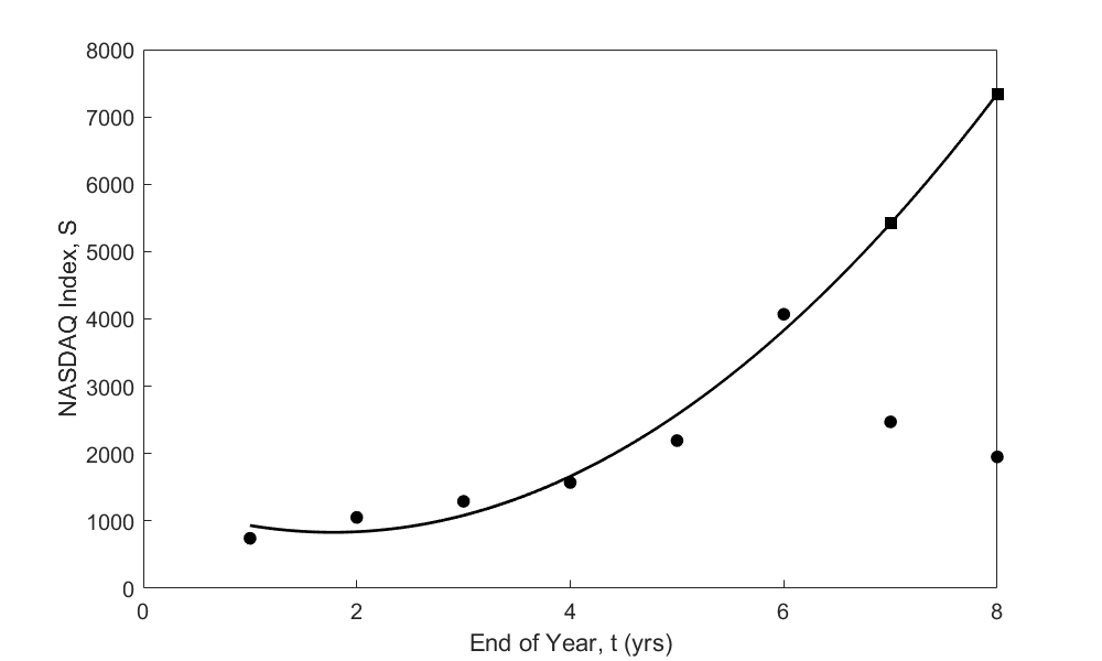
Figure 2 Extrapolated curve and actual data for Years 7 and 8.
Generalization
Generalization could arise when unsupported or exaggerated claims are made. It is not often possible to measure all predictor variables relevant in a study. For example, a study carried out about the efficacy of a drug might have inadvertently been restricted to men only. Shall we then generalize the result to be applicable to all? Such use of regression is an abuse since the limitations imposed by the data restrict the use of the prediction equations to men.
Misidentification
Finally, misidentification of causation is a classic abuse of regression analysis equations. Regression analysis can only aid in the confirmation or refutation of a causal model ‑ the model must, however, have a theoretical basis. In a chemical reacting system in which two species react to form a product, the amount of product formed or amount of reacting species vary with time. Although a regression equation of species concentration and time can be obtained, one cannot attribute time as the causal agent for the varying species concentration. Regression analysis cannot prove causality. Instead, it can only substantiate or contradict causal assumptions. Anything outside this is an abuse of the regression analysis method.
Multiple Choice Test
(1). For a linear regression model to be considered adequate, the percentage of scaled residuals that need to be in the range \(\lbrack - 2,2\rbrack\) is greater than or equal to
(A) \(5\%\)
(B) \(50\%\)
(C) \(90\%\)
(D) \(95\%\)
(2). Given \(20\) data pairs of \({y\;}\text{vs.}\ {x\ }\)data are regressed to a straight line. The straight line regression model is given by \(y = 9 - 5x\), and the coefficient of determination is found to be \(0.59\). The correlation coefficient is
(A) \(-0.7681\)
(B) \(-0.3481\)
(C) \(0.7681\)
(D) \(0.3481\)
(3). The following \(y \text{ vs. } x\) data is regressed to a straight line.
| \(x\) | \(5\) | \(6\) | \(7\) | \(8\) | \(9\) |
|---|---|---|---|---|---|
| \(y\) | \(0.3\) | \(0.4\) | \(0.57\) | \(0.6\) | \(1.77\) |
The linear regression model is found to be\(\ y = - 1.4700 + 0.3140x\). The coefficient of determination is
(A) \(0.3046\)
(B) \(0.4319\)
(C) \(0.6956\)
(D) \(0.8339\)
(4). Many times, you may not know what regression model to use for given discrete data. In such cases, a suggestion may be to use a polynomial model. But the question remains – what is the order of polynomial shoud I use? For example, if you are given \(10\) data points, you can regress the data to a polynomial order \(0,\ 1,\ 2,\ 3,\ 4,\ 5,\ 6,\ 7,\ 8,\) or \(9\). Below is the question you are asked to answer.
If \(S_{p}\) is the sum of the squares of the residuals for the regression polynomial model of order \(p\), the criterion you would use to find the optimum order of the polynomial would be to find the minimum of \(\displaystyle \frac{S_{p}}{m- p}\) for all possible polynomial orders. If you have \(30\) data points, then the value of \(m\) in the formula is
(A) \(10\)
(B) \(29\)
(C) \(30\)
(D) \(50\)
(5). On regressing \({n\ }\)data pairs \((x_{1},y_{1}),...,(x_{n},y_{n})\) to a linear regression model \(y = a_{0} + a_{1}x\), a scientist finds the regression model to have zero slope. The regression model then is given by
(A) \(\displaystyle y = \frac{\displaystyle\sum_{i = 1}^{n}x_{i}}{n}\)
(B) \(\displaystyle y = \frac{\displaystyle\sum_{i = 1}^{n}y_{i}}{n}\)
(C) \(y = 0\)
(D) \(\displaystyle y = \sqrt{\frac{\displaystyle \sum_{i = 1}^{n}{(y_{i} - \bar{y})^{2}}}{n - 1}}\)
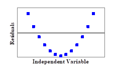
(6). Out of the following patterns of residuals, which one is the most acceptable for a linear regression model?
(A)
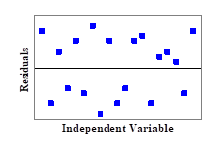
(B)
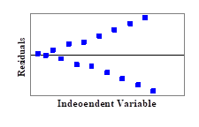
(C)
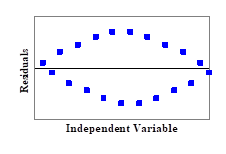
(D)
For complete solution, go to
http://nm.mathforcollege.com/mcquizzes/06reg/quiz_06reg_adequacy.pdf
Problem Set
(1). Water is flowing through a circular pipe of \(0.5 \text{ ft}\) radius, and flow velocity (\(\text{ft/s}\)) measurements are made from the center to the wall of the pipe as follows.
| \(\text{Radial location},\ r\ (\text{ft})\) | \(0\) | \(0.083\) | \(0.17\) | \(0.25\) | \(0.33\) | \(0.42\) | \(0.50\) |
|---|---|---|---|---|---|---|---|
| \(\text{Velocity},\ v (\text{ft/s})\) | \(10\) | \(9.72\) | \(8.88\) | \(7.5\) | \(5.6\) | \(3.1\) | \(0\) |
A scientist regresses the data to a straight line and is given by \(v(r) = - 19.92r + 11.39\).
a) How much is the absolute relative true error in the flow rate using the above velocity expression if the actual flow rate is \(3.9 \text{ft}^3/\text{s}\)?
b) Regress the data to a second-order polynomial of \(r\). What is the absolute relative true error for this case?
c) Regress the data to a specified second-order polynomial, \(v = a_{0}(1 - 4r^{2})\). Find the value of \(a_{0}\). What is the absolute relative true error in this case?
Answer: \(a)\ 3.7306\ \text{ft}^3/\text{s},\ 4.34\%\)
\(b)\ 3.9496\ \text{ft}^3/\text{s},\ 1.27\%\)
\(c)\ 3.9322\ \text{ft}^3/\text{s},\ 0.83\%\)
(2). The following \(y\) vs. \(x\) data is regressed to a straight line and is given by \(y = - 1.398 + 0.3x\).
| \(x\) | \(5\) | \(6\) | \(7\) | \(8\) | \(9\) |
|---|---|---|---|---|---|
| \(y\) | \(0.3\) | \(0.4\) | \(0.51\) | \(0.6\) | \(1.7\) |
Find the coefficient of determination.
Answer: \(0.69441\)
(3). Many times, you may not know what regression model to use for the given data. In such cases, a suggestion may be to use a polynomial. But the question remains, what is the order of the polynomial to use? For example, if you are given \(10\) data points, you can regress the data to a polynomial of order \(1,\ 2,\ 3,\ 4,\ 5,\ 6,\ 7,\ 8\) or \(9\). What order of polynomial would you use? An instructor suggests four different criteria. Only one is correct. Which one would you choose?
A) Find the sum of the square of residuals, \(S_{r}\) for all possible polynomials, and choose the order for which \(S_{r}\) is minimum.
B) Find \(\displaystyle \frac{\text{sum of the square of residuals}}{(\text{number of data points-order of polynomial})}\) for all possible polynomials and choose the order for which it is minimum.
C) Find \(\displaystyle \frac{\text{sum of the square of residuals}}{(\text{number of data points-order of polynomial - 1})}\) for all possible polynomials and choose the order for which it is minimum.
D) Find \(\displaystyle \frac{\text{sum of the square of residuals}}{(\text{number of data points-order of polynomial} + 1)}\) for all possible polynomials and choose the order for which it is minimum.
Answer: \((C)\)
(4). The following \(y\) vs. \(x\) data is regressed to a straight line and is given by \(y = - 1.398 + 0.3x\).
| \(x\) | \(5\) | \(6\) | \(7\) | \(8\) | \(9\) |
|---|---|---|---|---|---|
| \(y\) | \(0.3\) | \(0.4\) | \(0.51\) | \(0.6\) | \(1.7\) |
Find the scaled residuals and check how many of them are between in the range \([- 2,2].\)
Answer: All scaled residuals are in the range \([- 2,2].\)
(5). Water is flowing through a circular pipe of \(0.5\ \text{ft}\) radius, and flow velocity (\(\text{ft/s}\)) measurements are made from the center to the wall of the pipe as follows
| \(\text{Radial Location},\ r\ (\text{ft})\) | \(0\) | \(0.083\) | \(0.17\) | \(0.25\) | \(0.33\) | \(0.42\) | \(0.50\) |
|---|---|---|---|---|---|---|---|
| \(\text{Velocity},\ v\ (\ \text{ft/s})\) | \(10\) | \(9.72\) | \(8.88\) | \(7.5\) | \(5.6\) | \(3.1\) | \(0\) |
A scientist regresses the data to a straight line and is given by \(v(r) = - 19.92r + 11.39\). Verify if the model is adequate based on what you learned in class.
Answer: Make all four checks - residual plot characteristics may be a cause for rejection
(6). Water is flowing through a circular pipe of \(0.5\ \text{ft}\) radius, and flow velocity \((\text{ft/s})\) measurements are made from the center to the wall of the pipe as follows
| \(\text{Radial Location},\ r\ (\text{ft})\) | \(0\) | \(0.083\) | \(0.17\) | \(0.25\) | \(0.33\) | \(0.42\) | \(0.50\) |
|---|---|---|---|---|---|---|---|
| \(\text{Velocity},\ v\ ( \text{ft/s})\) | \(10\) | \(9.72\) | \(8.88\) | \(7.5\) | \(5.6\) | \(3.1\) | \(0\) |
Use an appropriate regression model to find the following.
a) Velocity at \(r = 0.3\ \text{ft}\).
b) Rate of change of velocity with respect to the radial location at \(r = 0.3\ \text{ft}\).
c) An engineer, who thinks they know everything, calculates the flow rate out of the pipe by averaging the given velocities and multiplying it by the cross-sectional area of the pipe. How will you convince them that they need to use a different (better) approach. Hint: The flow rate \(Q\) out of the pipe is given by the formula \(\displaystyle Q = \int_{0}^{0.5}{vdA} = \int_{0}^{0.5}{2\pi rvdr}\).
Answer: Use \(v=a(1-r^2/0.5^2)\)
\(a)\ 6.4082\ \text{ft/s},\)
\(b)\ -24.032\ \text{ft}^2/\text{s}\)
\(c)\) get \(5.0266 \ ft^3/s\) by average method, get \(3.9322 \ \text{ft}^3/\text{s}\) by using the integration formula
(7). For the purpose of shrinking a trunnion into a hub, the reduction of diameter, \(\Delta D\) of a trunnion shaft by cooling it through a temperature change of \(\Delta T\), is given by
\[\Delta D = D\int_{T_{\text{room}}}^{T_{\text{fluid}}}\alpha dT\]
where
\[D = \text{original diameter}\ (\text{in})\]
\[\alpha = \text{linear coefficient of thermal expansion}\ (\text{in/in/}^\circ \text{F})\]
\[T_{\text{fluid}} = \text{temperature of dry-ice/alcohol mixture,}\ (^\circ \text{F})\]
\[T_{\text{room}} = \text{room temperature,}\ (^\circ \text{F})\]
Given below is the table of the linear coefficient of thermal expansion vs. temperature
| Temperature (\(^\circ \text{F}\)) | Linear coefficient of thermal expansion coefficient (\(\mu in/in/^\circ \text{F}\)) |
|---|---|
| \(80\) | \(6.47\) |
| \(0\) | \(6.00\) |
| \(-60\) | \(5.58\) |
| \(-160\) | \(4.72\) |
| \(-260\) | \(3.58\) |
| \(-340\) | \(2.45\) |
A diametric contraction of \(0.015^{\prime\prime}\) is needed in the trunnion.
\[\text{Nominal outer diameter of the trunnion} =12.363^{\prime\prime}\]
\[\text{Temperature of dry-ice/alcohol mixture} =- 108^{\circ}\text{F}\]
\[\text{Temperature of liquid nitrogen} =- 321^{\circ}\text{F}\]
\[\text{Room temperature} =80^{\circ}\text{F}\]
a) Find the regression curve (a straight line is not acceptable) for the coefficient of linear thermal expansion as a function of temperature.
b) Find the diametric contraction of the trunnion if it is cooled in dry- ice/alcohol mixture? Can this cooling method be recommended to get the needed contraction?
c) If the answer to part (b) is no, would you recommend cooling it in liquid nitrogen? Why?
Answer: \(a)\ -0.1219\times 10^{-10}T^2+0.6313\times 10^{-8} T+0.6023\times 10^{-5}\)
\(b)\ 0.0137^{\prime\prime}\), not enough magnitude of contraction - cannot be recommended
\(c)\ 0.0244^{\prime\prime}\), enough magnitude of contraction - can be recommended