Chapter 01.03: Sources of Error
Learning Objectives
After successful completion of this lesson, you should be able to:
1) recognize that there are two inherent sources of error in numerical methods round-off and truncation error
2) define and exemplify round-off errors
Introduction
Error in solving an engineering or science problem can arise due to several factors. First, the error may be in the modeling technique. A mathematical model may be based on using assumptions that are not acceptable. For example, one may assume that the drag force on a car is proportional to the velocity of the car, but, actually it is proportional to the square of the velocity of the car. This itself can create huge errors in determining the performance of the car, no matter how accurate the numerical methods you may use. Second, errors may arise from mistakes in programs themselves or in the measurement of physical quantities. But, in applications of numerical methods themselves, the two errors we focus on are inherent to the subject, namely
1) round-off error
2) Truncation error.
What is a round-off error?
A computer can only represent a number approximately. For example, a number like \(\displaystyle \frac{1}{3}\) may be represented as \(0.333333\) on a PC. Then the round-off error, in this case, is
\(\displaystyle \frac{1}{3} - 0.333333 = 0.0000003\bar{3}\). Then there are other numbers that cannot be represented exactly. For example, \(\pi\) and \(\sqrt{2}\) are numbers that need to be approximated in computer calculations.
What problems can be created by round-off errors?
Round-off errors while storing numbers or while conducting arithmetic operations can propagate errors. Here is a real-life example of what happened when a small round-off error was responsible for a tragedy during the 1991 US-Iraq war.
Twenty-eight Americans were killed on February 25, 1991. An Iraqi Scud hit the Army barracks in Dhahran, Saudi Arabia. The Patriot defense system had failed to track and intercept the Scud. What was the cause of this failure?
The Patriot defense system consists of an electronic detection device called the range gate. It calculates the area in the air space where it should look for a Scud. To find out where it should aim next, it calculates the velocity of the Scud and the last time the radar detected the Scud. Time is saved in a register that has \(24\) bits in length. Since the internal clock of the system is measured for every one-tenth of a second, \(1/10\) is expressed in a \(24\) bit-register as \(0.00011001100110011001100\). However, this is not an exact representation. In fact, it would need infinite numbers of bits to represent \(1/10\) exactly. So, the error in the representation in decimal format is
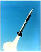
Figure 1 Patriot missile (Courtesy of the US Armed Forces,
(http://www.redstone.army.mil/history/archives/patriot/patriot.html)
\[\begin{split} \text{Error} &=\frac{1}{10} - (0 \times 2^{- 1} + 0 \times 2^{- 2} + 0 \times 2^{- 3} + 1 \times 2^{- 4} + ... + 1 \times 2^{- 22} + 0 \times 2^{- 23} + 0 \times 2^{- 24})\\ &= \frac{1}{10}-\frac{209715}{2097152} \\&= 9.537 \times 10^{- 8}\end{split}\]
The battery was on for 100 consecutive hours, hence causing an inaccuracy of
\[\begin{split} \text{Cumulative Error}&= 9.537 \times 10^{- 8}\frac{\text{s}}{0.1\ \text{s}} \times 100\text{ hr} \times \frac{3600\ \text{s}}{1\ \text{hr}}\\ &= 0.3433\ \text{s}\end{split}\]
The shift calculated in the range gate due to the error of \(0.342\ \text{s}\) was calculated as \(687\ \text{m}\). For the Patriot missile defense system, the target is considered out of range if the shift is more than than \(137\ \text{m}\). The shift of larger than \(137\ \text{m}\) resulted in the Scud not being targeted and hence killing 28 Americans in the barracks of Saudi Arabia.
Show an example of how not carrying enough significant digits can affect the solution to a problem?
In Table 1, the instantaneous coefficient of thermal expansion of steel is given as a discrete function of temperature.
Table 1: Instantaneous Coefficient of Linear Thermal Expansion vs. Temperature for Steel
| Temperature, T | Instantaneous Coefficient of Linear Thermal Expansion, \(\alpha\) |
|---|---|
| \(^{\circ}\text{F}\) | \(\mu\text{in/in/}^{\circ}\text{F}\) |
| \(80\) | \(6.47\) |
| \(60\) | \(6.36\) |
| \(40\) | \(6.24\) |
| \(20\) | \(6.12\) |
| \(0\) | \(6.00\) |
| \(-20\) | \(5.86\) |
| \(-40\) | \(5.72\) |
| \(-60\) | \(5.58\) |
| \(-80\) | \(5.43\) |
| \(-100\) | \(5.28\) |
| \(-120\) | \(5.09\) |
| \(-140\) | \(4.91\) |
| \(-160\) | \(4.72\) |
| \(-180\) | \(4.52\) |
| \(-200\) | \(4.30\) |
| \(-220\) | \(4.08\) |
| \(-240\) | \(3.83\) |
| \(-260\) | \(3.58\) |
| \(-280\) | \(3.33\) |
| \(-300\) | \(3.07\) |
| \(-320\) | \(2.76\) |
| \(-340\) | \(2.45\) |
Regression is used to develop a simple formula in the form of a second-order polynomial to relate the coefficient of thermal expansion coefficient of steel as a function of temperature.
Using Microsoft Excel and using its trend line function, it gives the formula as shown in Figure 2.
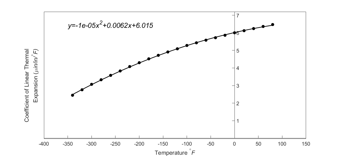
Figure 2: Regression Model with Default Format for Instantaneous Coefficient of Linear Thermal Expansion vs. Temperature for steel
The trend line given by Excel in its default format is
\[\alpha = - 1 \times 10^{- 5}T^{2} + 0.0062T + 6.015\;\;\;\;\;\;\;\;\;\;\;\; (1)\]
At
\[T = - 300{^\circ}\text{F},\]
the predicted value of the instantaneous coefficient of the thermal expansion from Equation (1) is
\[\begin{split} \alpha &= - 1 \times 10^{- 5}\left( - 300 \right)^{2} + 0.0062\left( - 300 \right) + 6.015\\ &=3.26\ \mu \text{in/in/}^{\circ} \text{F}\end{split}\]
From Table 1, the observed value
At
\[T = - 300{^\circ}\text{F} \text{ is}\]
\[\alpha = 3.07\ \mu\text{in/in}{/}^{\circ}\text{F}\]
which gives a residual at \(T = - 300{^\circ}\text{F}\) as
\[\begin{split} E_{i} &= 3.07 - 3.26\\ &= - 0.19\ \mu \text{in/in/}^{\circ}\text{F}\end{split}\;\;\;\;\;\;\;\;\;\;\;\; (2)\]
When a graduate student showed me the above numbers for the observed and predicted values, they did not match what was getting depicted in Figure 2. In the figure, the predicted value seemed much closer to the observed value than what is calculated above.
So what was the cause of this discrepancy? Notice that the default format setting for the trend line (Equation (1)) in Excel is the general format. But, now change the format setting to scientific format with say five significant digits, and we get the same trend line as
\[\alpha = - 1.2278 \times 10^{- 5}T^{2} + 6.1946 \times 10^{- 3}T + 6.0150\;\;\;\;\;\;\;\;\;\;\;\; (3)\]

Figure 3: Regression Model with Scientific Format for Instantaneous Coefficient of Linear Thermal Expansion vs. Temperature for steel
At
\[T = - 300{^\circ}\text{F},\]
the predicted value of the instantaneous coefficient of the thermal expansion from Equation (3)
\[\begin{split} \alpha &= - 1.2278 \times 10^{- 5}\left( - 300 \right)^{2} + 6.1946 \times 10^{- 3}\left( - 300 \right) + 6.0150\\ &= 3.05\ \mu\text{in/in}{/}^{\circ}\text{F} \end{split}\]
From Table 1, the observed value at
\[T = - 300{^\circ}\text{F} \]
is
\[\alpha = 3.07\ \mu\text{in/in}\text{/}^{\circ}\text{F}\]
which gives a residual of
\[\begin{split} E_{i} &= 3.07 - 3.05\\ &= 0.02\ \mu\text{in/in}{/}^{\circ}\text{F}\end{split}\;\;\;\;\;\;\;\;\;\;\;\; (4)\]
The residual now looks reasonable.
The difference between the predicted value (Equation(2) when using the default format of Excel
\[\alpha = 3.255\ \mu\text{in/in}{/}^{\circ}\text{F}\]
and the predicted value when using scientific format with \(5\) significant digits (Equation(4))
\[\alpha = 3.051\ \mu\text{in/in}{/}^{\circ}\text{F}\]
is attributed fully to the round-off error.
References
This reference is the full GAO report of the investigation that resulted after the accident. “Patriot Missile Defense – Software Problem Led to System Failure at Dhahran, Saudi Arabia”, GAO Report, General Accounting Office, Washington DC, February 4, 1992.
It should be pointed out that the Patriot missile was originally designed to be a mobile system and not used as an anti-ballistic system. In mobile systems, the clocks are reset more often. As per the article Operations: I Did Not Say You Could Do That! by Bill Barnes and Duke McMillin, here are some important observations: “It turns out that the original use case for this system was to be mobile and to defend against aircraft that move much more slowly than ballistic missiles. Because the system was intended to be mobile, it was expected that the computer would be periodically rebooted. In this way, any clock-drift error would not be propagated over extended periods and would not cause significant errors in range calculation. Because the Patriot system was not intended to run for extended times, it was probably never tested under those conditions—explaining why the problem was not discovered until the war was in progress. The fact that the system was also designed as an antiaircraft system probably also enabled the inclusion of such a design flaw because slower-moving airplanes would be easier to track and, therefore, less dependent upon a highly accurate clock value.”
Learning Objectives
After successful completion of this lesson, you should be able to:
1) define and exemplify truncation errors
2) recognize the difference between round-off and truncation error.
Introduction
Truncation error is defined as the error caused by approximating a mathematical procedure. Examples of mathematical procedure getting approximated include an infinite series where only the first few terms are used, integrals where the number of rectangles drawn to show the area under the curve is finite in number as opposed to infinite, and the derivative of a function is approximated by using the slope of a secant line as opposed to a tangent line.
Examples of Truncation Error
For example, the Maclaurin series for \(e^{x}\)is given as
\[ e^{x} = 1 + x + \frac{x^{2}}{2!} + \frac{x^{3}}{3!} + ... \;\;\;\;\;\;\;\;\;\;\;\; (1)\]
This series has an infinite number of terms, but when using this series to calculate \(e^{x}\), only a finite number of terms can be used. For example, if one uses three terms to calculate \(e^{x}\), then
\[ e^{x} \approx 1 + x + \frac{x^{2}}{2!}\]
the truncation error for such an approximation for any value of \(x\) is
\[\begin{split} \text{Truncation error} &= \ e^{x} - \left( 1 + x + \frac{x^{2}}{2!} \right)\\ &= \left( 1 + x + \frac{x^{2}}{2!} + \frac{x^{3}}{3!} + .... \right) - \left( 1 + x + \frac{x^{2}}{2!} \right)\\ &= \frac{x^{3}}{3!} + \frac{x^{4}}{4!} + .......................\end{split}\]
Example 1
Given the following infinite series, find the truncation error for \(x = 0.75\) if only the first three terms of the series are used.
\[S = 1 + x + x^{2} + x^{3} + \ldots,\ \left| x \right| < 1.\]
Solution
Using only the first three terms of the series for \(x=0.75\) gives
\[\begin{split} S_{3} &= \left( 1 + x + x^{2} \right)_{x = 0.75}\\ &= 1 + 0.75 + \left( 0.75 \right)^{2}\\ &=2.3125\end{split}\]
The sum of an infinite geometrical series
\[S = a + {ar} + {ar}^{2} + {ar}^{3} + \ldots,\ \left| r \right| < 1\]
is given by
\[S = \frac{a}{1 - r}\]
For our series, \(a = 1\) and \(r = 0.75\), to give
\[\begin{split} S &= \frac{1}{1 - 0.75}\\ &= 4\end{split}\]
The truncation error (\({TE}\)) hence is
\[\begin{split} {TE} &= 4 - 2.3125\\ &= 1.6875\end{split}\]
Example 2
Use the concept of the relative approximate error to illustrate through an example how truncation error can be controlled. Assume that you are not privy to the exact value.
Solution
Let us show through an example how many terms need to be considered in Equation (1) to calculate \(e^{1.2}\) within \(1\%\) pre-specified tolerance. Of course, you are not privy to the exact answer.
The summation series for \(e^{1.2}\) is given by
\[e^{1.2} = 1 + 1.2 + \frac{1.2^{2}}{2!} + \frac{1.2^{3}}{3!} + ...................\]
In Table 1, we tabulate the value of \(e^{1.2}\), approximate error and absolute relative approximate error as a function of the number of terms of the series used, \(n\).
Table 1: Values and approximate errors for \(e^{1.2}\) as a function of the number of terms of the Maclaurin series
| \(n\) | \(e^{1.2}\) | \(E_{a}\) | \(\displaystyle\left| \epsilon_{a} \right|\%\) |
|---|---|---|---|
| \(1\) | \(1\) | \(-\) | \(-\) |
| \(2\) | \(2.2\) | \(1.2\) | \(54.546\) |
| \(3\) | \(2.92\) | \(0.72\) | \(24.658\) |
| \(4\) | \(3.208\) | \(0.288\) | \(8.9776\) |
| \(5\) | \(3.2944\) | \(0.0864\) | \(2.6226\) |
| \(6\) | \(3.315136\) | \(0.020736\) | \(0.6255\) |
Using a minimum of \(6\) terms of the series yields an absolute relative approximate error \(\left| \epsilon_{a} \right|< 1\%\). The reported value of \(e^{1.2}\) is \(3.3151\) and is shown up to \(5\) significant digits. As a side note, the exact value, up to \(5\) significant digits, of \(e^{1.2}\) is \(3.3201\).
Learning Objectives
After successful completion of this lesson, you should be able to:
1) exemplify truncation errors through numerical differentiation and integration
Can you give me other examples of truncation errors?
In many textbooks on numerical methods, the Maclaurin series is used as the only example to illustrate truncation error. This example may lead you to believe that truncation errors are just a result of using a finite number of terms of the series. However, truncation errors take place in other mathematical procedures as well. In this lesson, we take two such examples.
Example 1
To find the exact derivative of a function, we define
\[f^{\prime}\left( x \right) = \lim_{h \rightarrow 0}\frac{f\left( x + h \right) - f\left( x \right)}{h}\]
But since we cannot use \(h \rightarrow 0\), in numerical methods, we use a finite value of \(h\), to give
\[f^{\prime}(x) \approx \frac{f(x + h) - f(x)}{h}\]
So the truncation error is caused by choosing a finite value of \({h }\) as opposed to a \(h \rightarrow 0.\)
Find the truncation error for finding \(f^{\prime}(3)\) for \(f(x) = x^{2}\) using a step size of \(h = 0.2\)
Solution
In finding \(f^{\prime}(3)\) for \(f(x) = x^{2}\), we have the exact value of the derivative calculated as follows. Given
\[f(x) = x^{2}\]
from the definition of the derivative of a function,
\[\begin{split} f^{\prime}(x) &= \lim_{h \rightarrow 0}\frac{f(x + h) - f(x)}{h}\\ &= \lim_{h \rightarrow 0}\frac{(x + h)^{2} - (x)^{2}}{{\Delta x}}\\ &= \lim_{h \rightarrow 0}\frac{x^{2} + 2xh + h^{2} - x^{2}}{{\Delta x}}\\ &= \lim_{h \rightarrow 0}(2x + h)\\ &= 2x\end{split}\]
The above derivative is the same expression you would have obtained by directly using the formula from your differential calculus class
\[ \frac{d}{{dx}}(x^{n}) = nx^{n - 1}\]
By this formula for
\[f(x) = x^{2}\]
\[f^{\prime}(x) = 2x\]
The exact value of \(f^{\prime}(3)\) is
\[\begin{split} f^{\prime}(3) &= 2 \times 3\\ &= 6\end{split}\]
Given the step size of \(h = 0.2\), we get
\[\begin{split} f^{\prime}(3) &= \frac{f(3 + 0.2) - f(3)}{0.2}\\ &= \frac{f(3.2) - f(3)}{0.2}\\ &= \frac{3.2^{2} - 3^{2}}{0.2}\\ &= \frac{10.24 - 9}{0.2}\\ &= \frac{1.24}{0.2}\\ &= 6.2\end{split}\]
\[\begin{split} \text{Truncation Error} &= \text{Exact Value} - \text{Approximate Value}\\ &= 6 - 6.2\\ &= -0.2\end{split}\]
Note: The example purposefully chose a simple function \(f(x) = x^{2}\) with the value of \(x = 2\) and \(h = 0.2\) because we wanted to have no round-off error in our calculations so that the truncation error is the only error in the example.
Question: Can you reduce the truncation error by choosing a smaller \(h\)?
Example 2
Another example of truncation error is the numerical integration of a function,
\[I = \int_{a}^{b}{f(x)dx}\]
Exact calculations require us to calculate the area under the curve by adding the area of the rectangles, as shown in Figure 1. However, exact calculations would require an infinite number of such rectangles. Since we cannot choose an infinite number of rectangles, we will have a truncation error.
For the integral
\[\int_{3}^{9}x^{2}{dx}\]
find the truncation error if a two-segment left-hand Reimann sum with equal width of segments is used.
Solution
We have the exact value as
\[\begin{split} \int_{3}^{9}{x^{2}{dx}} &= \left\lbrack \frac{x^{3}}{3} \right\rbrack_{3}^{9}\\ &= \left\lbrack \frac{9^{3} - 3^{3}}{3} \right\rbrack\\ &= 234 \end{split}\]
Using two rectangles of equal width to approximate the area (see Figure 1) under the curve, the approximate value of the integral
\[\begin{split} \int_{3}^{9}{x^{2}{dx}} &\approx \left. \ (x^{2}) \right|_{x = 3}(6 - 3) + \left. \ (x^{2}) \right|_{x = 6}(9 - 6)\\ &= (3^{2})3 + (6^{2})3\\ &= 27 + 108\\ &= 135\end{split}\]
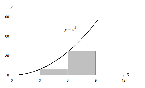
Figure 1 Plot of \(y = x^{2}\) showing the approximate area under the curve from \(x = 3\) to \(x = 9\) using two rectangles.
\[\begin{split} \text{Truncation Error} &= \text{Exact Value} - \text{Approximate Value}\\ &= 234 - 135\\ &=99.\end{split}\]
Note: Again, we purposefully chose a simple example with such numbers to produce numbers without round-off error in our calculations. This deliberate choice makes the obtained error purely due to truncation.
Question: Can you reduce the truncation error by choosing more rectangles as given in Figure 2? What is the truncation error when four rectangles are chosen?
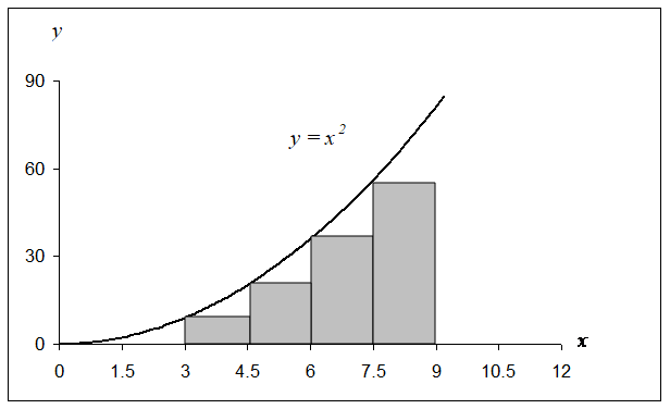
Figure 2 Plot of \(y = x^{2}\) showing the approximate area under the curve from \(x = 3\) to \(x = 9\) using four rectangles.
Multiple Choice Test
(1). Truncation error is caused by approximating
(A) irrational numbers
(B) fractions
(C) rational numbers
(D) exact mathematical procedures.
(2). A computer that represents only \(4\) significant digits with chopping would calculate \(66.666\times33.333\) as
(A) \(2220\)
(B) \(2221\)
(C) \(2221.17778\)
(D) \(2222\)
(3). A computer that represents only 4 significant digits with rounding would calculate \(66.666\times33.333\) as
(A) \(2220\)
(B) \(2221\)
(C) \(2221.17778\)
(D) \(2222\)
(4). The truncation error in calculating \(f^\prime\left( 2 \right)\) for \(f\left( x \right) = x^{2}\) by \(\displaystyle f^{\prime}\left( x \right) \approx \frac{f\left( x + h \right) - f\left( x \right)}{h}\) with \(h = 0.2\) is
(A) \(-0.2\)
(B) \(0.2\)
(C) \(4.0\)
(D) \(4.2\)
(5). The truncation error in finding \(\displaystyle \int_{- 3}^{9}{x^{3}{dx}}\) using LRAM (left end point Riemann approximation method) with equally portioned points \(- 3 < 0 < 3 < 6 < 9\) is
(A) \(648\)
(B) \(756\)
(C) \(972\)
(D) \(1620\)
(6). The number \(\displaystyle \frac{1}{10}\) is registered in a fixed \(6\) bit-register with all bits used for the fractional part. The difference is accumulated every \(\displaystyle \frac{1}{10}\)th of a second for one day. The magnitude of the accumulated difference is
(A) \(0.082\)
(B) \(135\)
(C) \(270\)
(D) \(5400\)
For complete solution, go to
http://nm.mathforcollege.com/mcquizzes/01aae/quiz_01aae_sourceserror_answers.pdf
Problem Set
(1). What is the round-off error in representing 200/3 in a 6-significant digit computer that chops the last significant digit?
Answer: \(0.00006666666....\)
(2). What is the round-off error in representing 200/3 in a 6-significant digit computer that rounds off the last significant digit?
Answer: \(-0.00003333333...\)
(3). What is the truncation error in the calculation of the \(f^{\prime}(x)\) that uses the approximation
\[f^{\prime}(x) \approx \frac{f(x + \Delta x) - f(x)}{\Delta x}\]
for
\[f(x) = x^{3},\ \Delta x = 0.4,\ \text{and}\ x = 5\]
Answer: \(-6.16\)
(4) What is the truncation error in the calculation of \(\displaystyle \sin (\frac{\pi}{2})\) if only first five terms of the Maclaurin series are used for the calculation? Ignore the round-off error in your calculations.
\[\sin(x) = x - \frac{x^{3}}{3!} + \frac{x^{5}}{5!} - \frac{x^{7}}{7!} + ......\]
Answer: \(-0.35427560\times10^{-5}\)
(5). The integral \(\displaystyle\int_{3}^{9}{x^{2}{dx}}\) can be calculated approximately by finding the area of the four rectangles as shown in Figure 1. What is the truncation error due to this approximation?
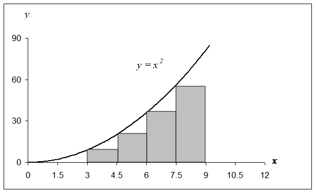
Figure 1 Plot of \(y = x^{2}\) showing the approximate area under the curve from \(x = 3\) to \(x = 9\) using four rectangles.
Answer: \(51.75\)
(6). Below is the data given for linear coefficient of thermal expansion for steel as a function of temperature.
| Temperature | Instantaneous Thermal Expansion Coefficient |
|---|---|
| \(^{\circ} \text{F}\) | \(\mu \text{in/in/}^{\circ}\text{F}\) |
| \(80\) | \(6.47\) |
| \(60\) | \(6.36\) |
| \(40\) | \(6.24\) |
| \(20\) | \(6.12\) |
| \(0\) | \(6.00\) |
| \(-20\) | \(5.86\) |
| \(-40\) | \(5.72\) |
| \(-60\) | \(5.58\) |
| \(-80\) | \(5.43\) |
| \(-100\) | \(5.28\) |
| \(-120\) | \(5.09\) |
| \(-140\) | \(4.91\) |
| \(-160\) | \(4.72\) |
| \(-180\) | \(4.52\) |
| \(-200\) | \(4.30\) |
| \(-220\) | \(4.08\) |
| \(-240\) | \(3.83\) |
| \(-260\) | \(3.58\) |
| \(-280\) | \(3.33\) |
| \(-300\) | \(3.07\) |
| \(-320\) | \(2.76\) |
| \(-340\) | \(2.45\) |
Regression is used to come up with a simple formula – a second order polynomial to relate the linear coefficient of thermal expansion of steel as a function of temperature.
a) The formula given by MS Excel using default settings is shown in Figure 2. Using the formula, what is the value of the linear coefficient of thermal expansion at \(T = - 300\), \(-200\), \(- 100\), \(0\) and \(100^\circ \text{F}\)? Compare these values with those given in the table above.

Figure 2 Default trend line given by excel
(b) Now the default settings for the trend line (Figure 3) are changed to scientific format with five significant digits. Using the formula, what is the value of linear coefficient of thermal expansion at \(T = - 300\), \(- 200\),\(- 100\), \(0\) and \(100^\circ \text{F}\)? Compare these values with those given in the table above.
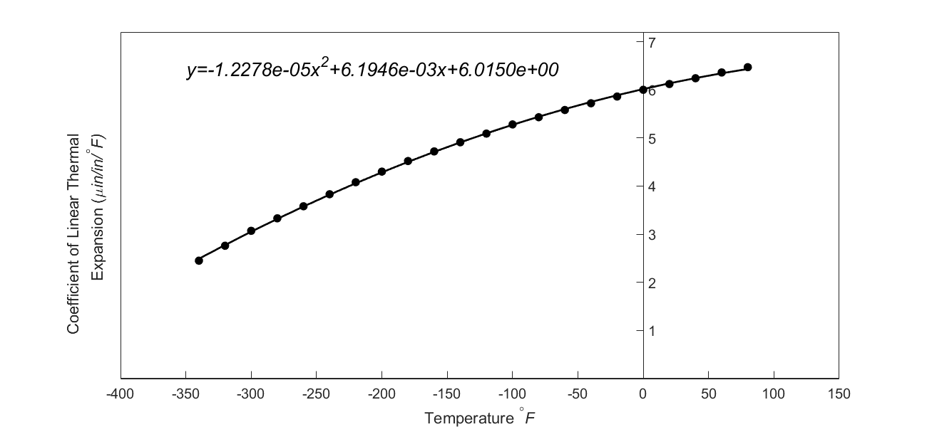
Figure 3 Trend line given by Excel using scientific format.
c) Do you get different answers in part (a) and part (b) for the predicted value of the linear coefficient of thermal expansion at \(T = - 300^{\circ}\text{F}\)? Yes or No.
d) In part (c), what do you attribute the difference or lack of difference in answers to?
Answer: a) At \(T=-300^{\circ}\text{F}\), \(\alpha=3.255 \text{ in/in/}^{\circ}\text{F}\). From table, \(\alpha=3.07 \text{ in/in/}^{\circ}\text{F}\) b) At \(T=-300^{\circ}\text{F}\), \(\alpha=3.0516 \text{ in/in/}^{\circ}\text{F}.\) From table, \(\alpha=3.07 \text{ in/in/}^{\circ}\text{F}\) c) No d) Answer not given intentionally.