Chapter 05.10: Length of a Curve
Learning Objectives
After successful completion of this lesson, you should be able to:
1) estimate the length of a curve given by a continuous function,
2) estimate the length of a curve found by interpolation of discrete data points.
Introduction
The length, \(L\) of a smooth function \(y(x)\) from \((a,f(a))\ to\ (b,f(b))\)is given analytically by (Figure 1)
\[L = \int_{a}^{b}{\sqrt{1 + \left( \frac{{dy}}{{dx}} \right)^{2}}{dx}}\;\;\;\;\;\;\;\;\;\;\;\; (1)\]
Over the interval \(\lbrack a,b\rbrack\), the integrand is required to be integrable, \(y(x)\) needs to be differentiable, and \(y'(x)\) has to be continuous. The length can be thought of as the distance one would travel if traversing along the path of the curve. An application would be to calculate the length of the path traversed by a robot that moves from one point to another on a continuous curve.
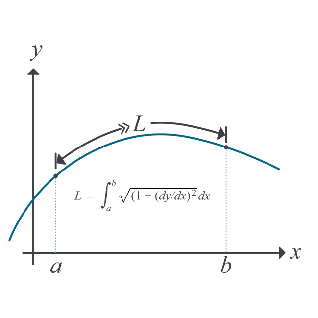
Figure 1. Length of a curve.
Example 1
Plot the function\(\displaystyle \ y = \frac{1}{3}(x^{2} + 2)^{\frac{3}{2}}\) and find the length of the curve from \(x = 0\) to \(x = 3\).
Solution
We use the equation
\[L = \int_{a}^{b}{\sqrt{1 + \left( \frac{{dy}}{{dx}} \right)^{2}}{dx}}\;\;\;\;\;\;\;\;\;\;\;\; (E1.1) \]
We have
\[y = \frac{1}{3}(x^{2} + 2)^{\frac{3}{2}}\]
So,
\[\begin{split} \frac{{dy}}{{dx}} &= \left( \frac{1}{3} \right) \times \left( \frac{3}{2} \right) \times \left( x^{2} + 2 \right)^{\frac{3}{2}\ - 1} \times \left( 2x \right)\\ &= x\sqrt{x^{2} + 2} \end{split} \;\;\;\;\;\;\;\;\;\;\;\; (E1.2) \]
Substituting Equation (E1.2) in Equation (E1.1), the length of the curve from \(x = 0\) to \(x = 3\) is
\[\begin{split} L &= \int_{0}^{3}{\sqrt{1 + \left( x\sqrt{x^{2} + 2} \right)^{2}}{dx}}\\ &= \int_{0}^{3}{\sqrt{1 + x^{2}\left( x^{2} + 2 \right)}{dx}}\\ &= \int_{0}^{3}{\sqrt{1 + x^{4} + 2x^{2}}{dx}}\\ &= \int_{0}^{3}{\sqrt{\left( x^{2} + 1 \right)^{2}}{dx}}\\ &= \int_{0}^{3}{(x^{2} + 1){dx}}\\ &= \left\lbrack \frac{x^{3}}{3} + x \right\rbrack\begin{matrix} 3 \\ \\ 0 \\ \end{matrix}\\ &= 12 \end{split}\]
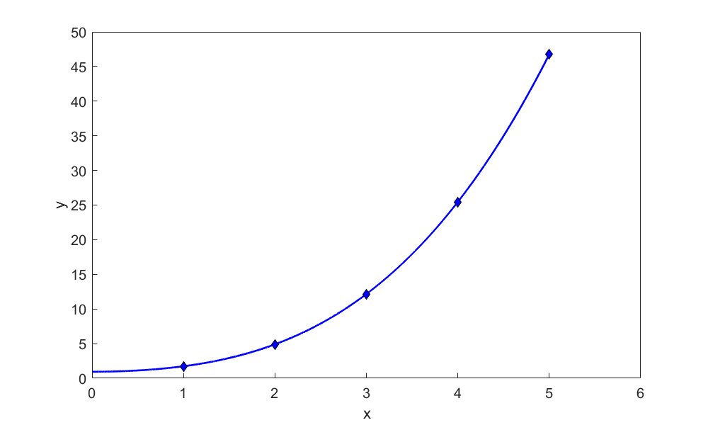
Figure 2. Plot of the function \(\displaystyle y = \frac{1}{3}(x^{2} + 2)^{\frac{3}{2}}\)
Example 2
A function passes consecutively through the three points \({(2,8),~(4,18),~(8,5)}\) and is found by as a \(2^{nd}\) order polynomial interpolant.
a) Find the function.
b) Find the approximate length of the function from \(x = 2\) to \(x = 8\). You can use the Simpson’s \(1/3^{rd}\) rule of integration rule as given by
\[\int_{a}^{b}{f(x)dx} \approx \frac{(b - a)}{6}\left\lbrack f(a) + 4f\left( \frac{a + b}{2} \right) + f(b) \right\rbrack\]
c) What is the absolute relative true error for part (b) if the exact length from \((2,8)\) to \((8,5)\) of the second-order polynomial is \(26.042\)?
Solution
a) The second-order interpolant is given by
\[y = a_{0} + a_{1}x + a_{2}x^{2}\]
Since it passes through \({(2,8), (4,18), (8,5)}\), we can set up three equations as
\[\begin{split} a_{0} + a_{1}2 + a_{2}2^{2} &= 8\\ a_{0} + a_{1}4 + a_{2}4^{2} &= 18\\ a_{0} + a_{1}8 + a_{2}8^{2} &= 5\end{split}\;\;\;\;\;\;\;\;\;\;\;\; (E2.1-E2.3)\]
Solving Equations (E2.1), (E2.2), (E2.3) simultaneously gives
\[a_{0} = - 13,\ a_{1} = 13.25,\ a_{2} = - 1.375\]
The resulting interpolant is
\[y = - 13 + 13.25x - 1.375x^{2}\;\;\;\;\;\;\;\;\;\;\;\; (E2.4)\]
b) The length of the curve \(y\left( x \right)\) from \(a\) to \(b\) is given by
\[L = \int_{a}^{b}{\sqrt{1 + \left( \frac{{dy}}{{dx}} \right)^{2}}{d}x} \;\;\;\;\;\;\;\;\;\;\;\; (E2.5)\]
Since
\[y = - 13 + 13.25x - 1.375x^{2}\]
\[\begin{split}\frac{dy}{dx}&= \frac{d}{dx}(- 13 + 13.25x - 1.375x^2)\\ &= 13.25- 1.375(2x) \\ &= 13.25-2.75x\end{split}\;\;\;\;\;\;\;\;\;\;\;\; (E2.6)\]
Substituting Equation (E2.6) in Equation (E2.5), the length of the curve from \(x = 2\) to \(x = 8\) is given by
\[L = \int_{2}^{8}{\sqrt{1 + \left( 13.25 - 2.75x \right)^{2}}{d}x}\;\;\;\;\;\;\;\;\;\;\;\; (E2.7)\]
Recall from the problem statement of part (b), integral given by Equation (E2.7) is asked to be found approximately by using Simpson’s 1/3rd rule, that is,
\[\int_{a}^{b}{f(x)dx} \approx \frac{(b - a)}{6}\left\lbrack f(a) + 4f\left( \frac{a + b}{2} \right) + f(b) \right\rbrack\]
In this case
\[f\left( x \right) = \sqrt{1 + \left( 13.25 - 2.75x \right)^{2}\ },\ a = 2,\ b = 8\]
Hence Equation (E2.7) gives
\[\begin{split}L & = \int_{2}^{8}{f(x)dx} \\ &\approx \frac{(8 - 2)}{6}\left\lbrack f(2) + 4f\left( \frac{2 + 8}{2} \right) + f(8) \right\rbrack\\ &= f(2) + 4f\left( 5 \right) + f(8)\\ &= 7.814 + 4\left( 1.118 \right) + 8.807\\ &= 21.093\end{split}\]
c) \[\text{True value } = 26.042\]
\[\text{Approximate value } = 21.093\]
So the absolute relative true error is
\[\begin{split} \left| \epsilon_{t} \right| &= \left| \frac{\text{True value} - \text{Approximate value}}{\text{True value}} \right| \times 100\\ &= \left| \frac{26.042 - 21.093\ }{26.042} \right| \times 100\\ &= 19.003 \% \end{split}\]
Learning Objectives
After successful completion of this lesson, you should be able to:
1) find the shortest smooth path through consecutive points, and
2) compare the lengths of different paths.
Introduction
In the previous lesson, you learned how to find the length of a curve numerically. In this lesson, via an example, we apply what we learned to find the shortest but smoothest path to go through consecutive points.
Example 1
Peter: “Dr. Kaw, I am taking a course in manufacturing. We are solving the following problem. A robot arm with a rapid laser is used to do a quick quality check, such as the radius of hole, on six holes on a rectangular plate \(15^{\prime\prime} \times 10^{\prime\prime}\) at several points as shown in Table 1 and Figure 1.
Table 1 The coordinate values of six holes on a rectangle plate.
| \(x\) | \(y\) |
|---|---|
| \(2.00\) | \(7.2\) |
| \(4.5\) | \(7.1\) |
| \(5.25\) | \(6.0\) |
| \(7.81\) | \(5.0\) |
| \(9.20\) | \(3.5\) |
| \(10.60\) | \(5.0\) |
I am using Excel to fit a fifth-order polynomial through the 6 points. But, when I plot the polynomial, it is taking a long path! (Figure 2)”
Kaw: “Why do you not just join the consecutive points by a straight line, just like the kids do at Pizza Hut™ with those ‘Connect the dots’ activities?”
Peter: “You are making me hungry, and I wish it were that easy. The path of the robot going from one point to another point needs to be smooth so as to avoid sharp jerks in the arm that can otherwise create premature wear and tear of the robot arm.”
Kaw: “As I recall, you took my course in Numerical Methods. What was that …… one year ago?”
Peter: “Yes, your memory is sharp, but my retention from that course – can we not talk about that?!?”
Kaw: “Come into my office. I wrote this program using Maple. See this function, \(f(x)=1/(1+25x^2)\). I am choosing \(7\) points equidistantly (Table 2) between \(-1\) and \(1\).
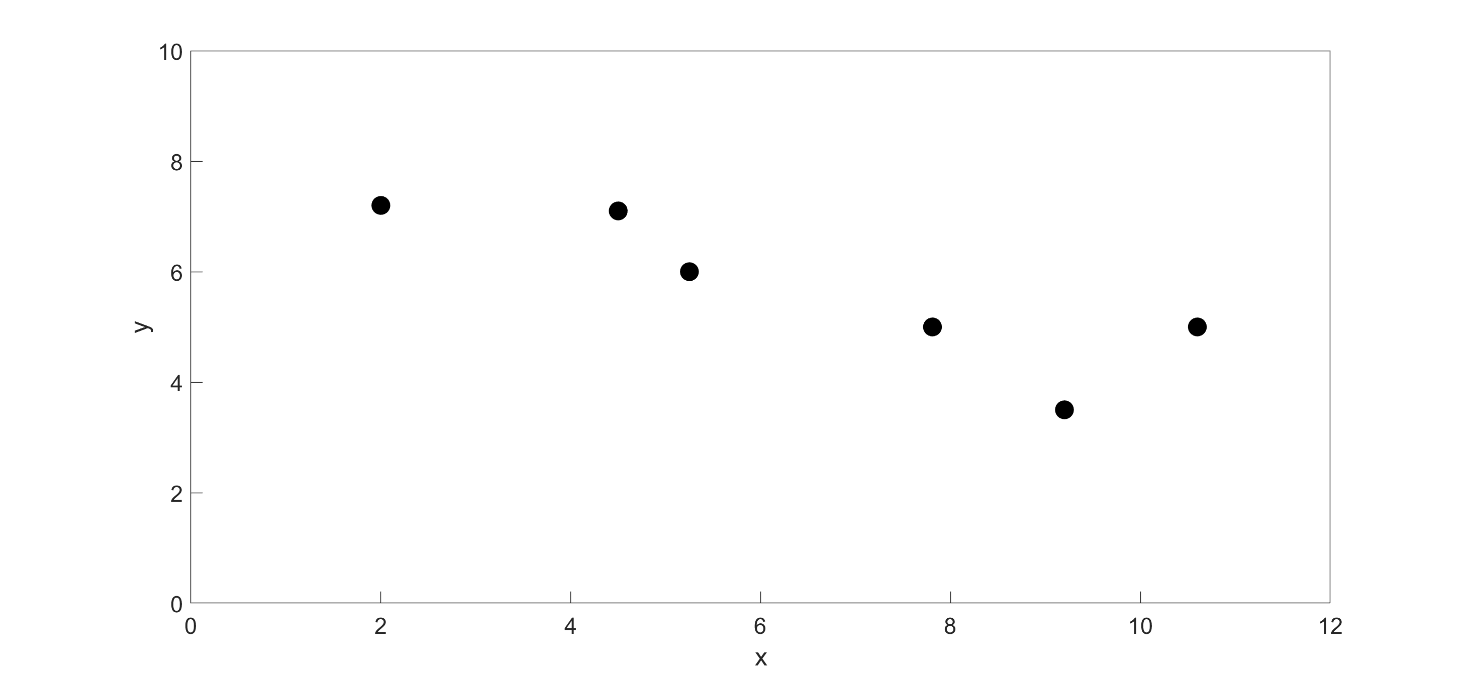
Figure 1 Locations of holes on the rectangular plate.
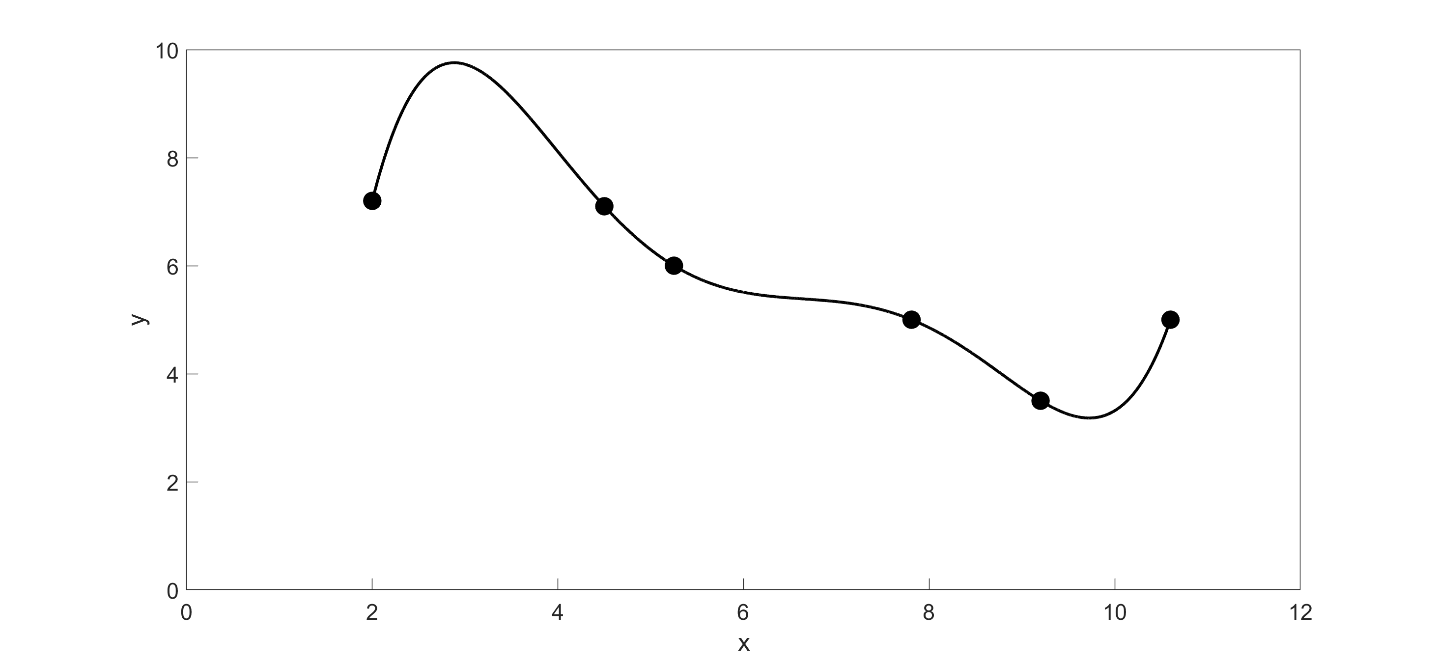
Figure 2 Approximating the path of the robot using 5th order polynomial.
Now, look at the sixth order interpolating polynomial and the original function (Figure 3). See the oscillations in the interpolating polynomial. In 1901, Runge used this example function to show that higher-order interpolation is a bad idea. One of the solutions to your robot path problem is to use quadratic or cubic spline interpolation. That gives a smooth curve with fewer oscillations and a smoother and shorter path.”
Table 2 The coordinate values of 7 equidistantly spaced points.
| \(x\) | \(\displaystyle y = \frac{1}{1+25x^2}\) |
|---|---|
| \(-1\) | \(0.038462\) |
| \(-0.66667\) | \(0.0826\) |
| \(-0.33333\) | \(0.264706\) |
| \(0\) | \(1\) |
| \(0.333333\) | \(0.264706\) |
| \(0.666667\) | \(0.082569\) |
| \(1\) | \(0.0385\) |
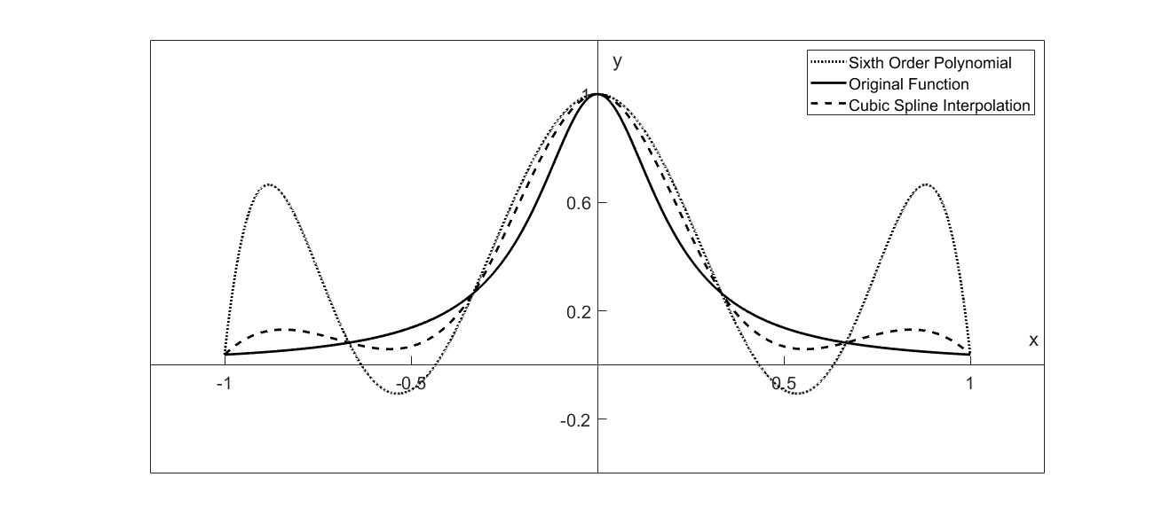
Figure 3 Runge’s function interpolated.
Peter: “Okay. Let’s give that a try.”
Kaw: “Now, let’s try generating a set of cubic splines to go through the data:”
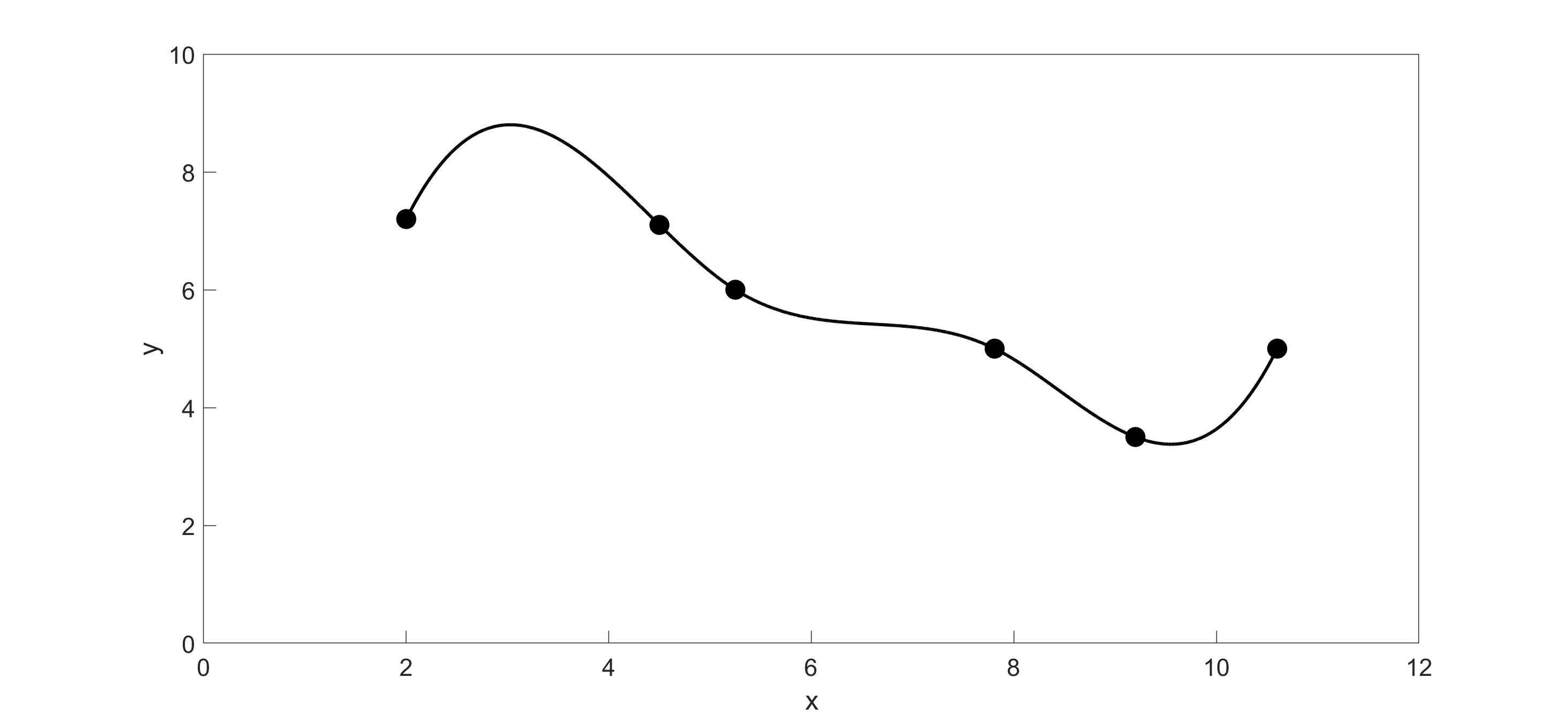
Figure 4 Path of the robot arm using cubic spline interpolation.
Peter: “Wow! That (Figure 4) looks much better!”
Kaw: “It may look better, but let’s find out for sure. See if you can combine the two plots (Figure 5) and compare the lengths of each path.”
Peter: “The length of a path if from to is given by
\[S=\int_{a}^{b}\sqrt{1+\left(\frac{df}{dx}\right)^2}dx\;\;\;\;\;\;\;\;\;\;\;\; (1)\]
Right?”
Table 3 Comparison of the length of curves.
| Type of interpolation | 5th order polynomial | Cubic Spline |
|---|---|---|
| Length of Curve | \(14.919^{\prime\prime}\) | \(11.248^{\prime\prime}\) |
Kaw: “Yes! You solved the problem. See Table 3 for answers.”
Peter: “I guess your class was good for something, after all, Dr. Kaw.”
Kaw: “Are you sure? You could have always fallen back on the connecting-the-dots method. Besides, you don’t want to grow up … you’re a Pizza Hut™ kid, right?”
Peter: “No, that’s a Toys R’ Us™ kid.”
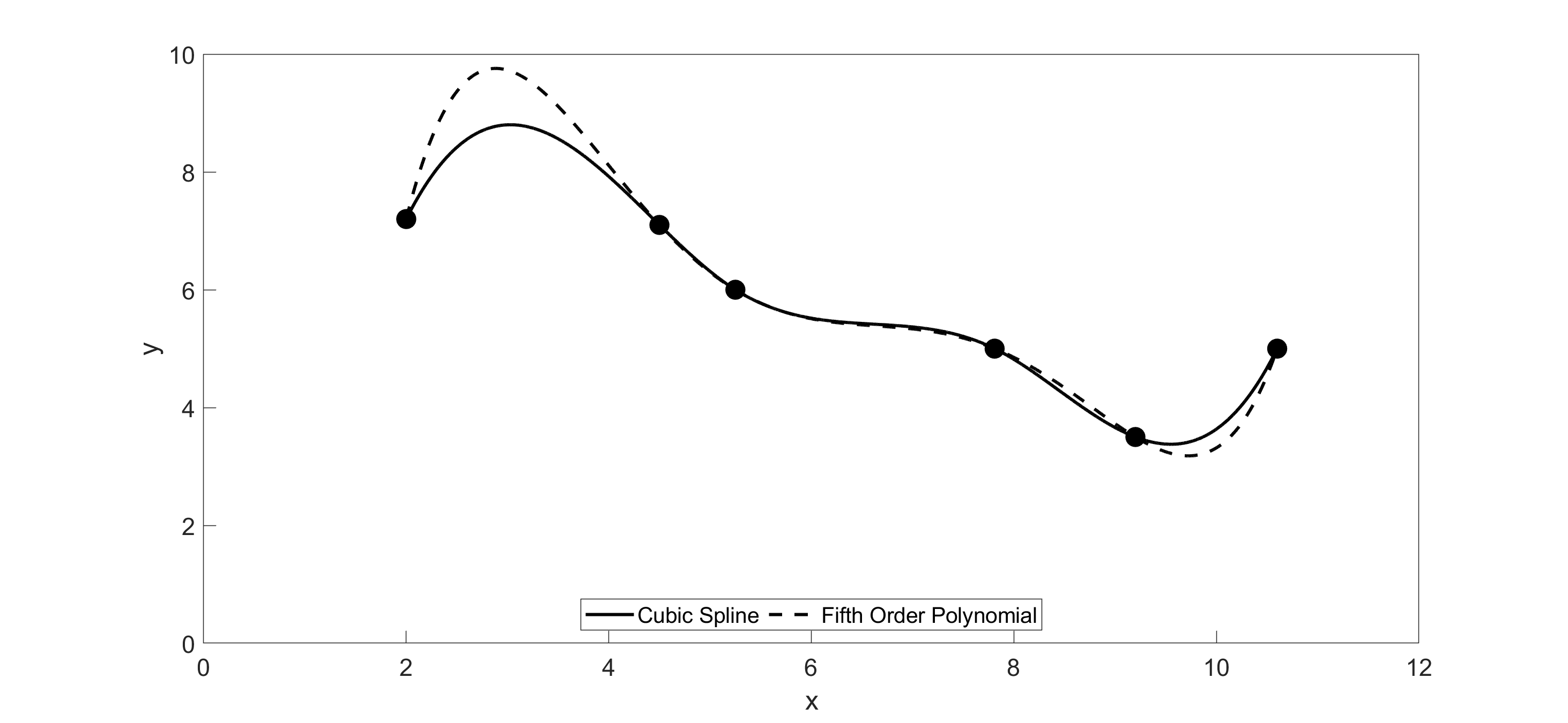
Figure 5 Path of robot arm compared using polynomial interpolation and cubic spline interpolation.
Multiple Choice Test
(1). The arc length of a smooth cartesian curve \(f(x)\) from \(a\) to \(b\) is given by
(A) \(\displaystyle \int_{a}^{b}{f\left( x \right){dx}}\)
(B) \(\displaystyle {(b - a)}^{2} + {(f\left( b \right) - f\left( a \right))}^{2}\)
(C) \(\displaystyle \int_{a}^{b}\sqrt{\left( 1 + \frac{{d}y}{{d}x} \right)}{dx}\)
(D) \(\displaystyle \int_{a}^{b}\sqrt{\left( 1 + \left( \frac{{d}y}{{d}x} \right)^{2} \right)}{dx}\)
(2). Which of these definite integrals gives the length of the arc of the function
\(f\left( x \right) = 3x + \sin x\) from \(x = 2\) to \(x = 5\)
(A) \(\displaystyle \int_{2}^{5}{(3x + \sin x){dx}}\)
(B) \(\displaystyle \int_{2}^{5}{\sqrt{1 + (3 + \cos x)}{dx}}\)
(C) \(\displaystyle \int_{2}^{5}{\sqrt{1 + {(3 + \cos x)}^{2}}{dx}}\)
(D) \(\displaystyle \int_{2}^{5}{\sqrt{1 + {(3x + \sin x)}^{2}}{dx}}\)
(3). The length of the curve \(y = \sqrt{1 - x^{2}}\) from \(x = 0\) to \(x = 1\) is most nearly equal to
(A) \(0.7854\)
(B) \(1.414\)
(C) \(1.518\)
(D) \(1.571\)
(4). A robotic drawing pencil is using linear spline interpolation to trace a path consecutively through three data points \((4,20)\), \((6,10)\), and \((9,25)\). What is the length of the path that the pencil traces if it begins at the first data point and ends at the last data point?
(A) \(15.297\)
(B) \(10.198\)
(C) \(7.071\)
(D) \(25.495\)
(5). A path is traversed consecutively through three points \((2,4)\), \((5,11)\), \((8,3)\) using a quadratic polynomial. Estimate the exact length of the path up to at least \(4\) significant digits. Use only MATLAB or some other program to do this problem - do not do it manually as it will take time.
(A) \(16.701\)
(B) \(6.0827\)
(C) \(16.160\)
(D) \(51.387\)
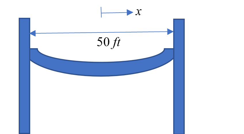
(6). A cable hangs between two poles that are \(50\) feet apart. The shape of the cable is given by
\[f\left( x \right) = a\cosh\left( \frac{x}{a} \right),\ - 25 \leq x \leq 25,\]
where \(a\) is dependent on the tension in the cable and the weight per unit length of the cable, and \(x\) is measured between the poles but from the center of the cable. If the length of the cable is 60 feet, the formula that will allow us to find the value of \(a\) is
(A) \(\displaystyle {\ 2\ a^{2}\sinh}\left( \frac{25}{a} \right) = 60\)
(B) \(\displaystyle {\ 2\ a{\ sinh}}\left( \frac{25}{a} \right) = 60\)
(C) \(\displaystyle {\ 2\ a{\ sinh}}\left( \frac{25}{a} \right) = 50\)
(D) \(\displaystyle {\ 2\ a^{2}\sinh}\left( \frac{25}{a} \right) = 50\)