Chapter 08.05: On Solving Higher-Order and Coupled Ordinary Differential Equations
Learning Objectives
After successful completion of this lesson, you should be able to:
1) write higher-order ordinary differential equations as simultaneous first-order ordinary differential equations,
2) solve higher-order ordinary differential equations numerically
Description
In the earlier lessons, we have learned Euler’s and Runge-Kutta methods to solve first-order ordinary differential equations of the form
\[\frac{{dy}}{{dx}} = f\left( x,y \right),y\left( x_{0} \right) = y_{0}\;\;\;\;\;\;\;\;\;\;\;\; (1)\]
What do we do to solve simultaneous (coupled) differential equations or differential equations higher than first order? For example, an \(n^{{th}}\)order differential equation of the form
\[a_{n}\frac{d^{n}y}{dx^{n}} + a_{n - 1}\frac{d^{n - 1}y}{dx^{n - 1}} + \ldots + a_{1}\frac{{dy}}{{dx}} + a_{o}y = f\left( x \right)\;\;\;\;\;\;\;\;\;\;\;\; (2)\]
with \(n\) initial conditions can be solved by assuming
\[y = z_{1}\;\;\;\;\;\;\;\;\;\;\;\; (3.1)\]
\[\frac{{dy}}{{dx}} = \frac{dz_{1}}{{dx}} = z_{2}\;\;\;\;\;\;\;\;\;\;\;\; (3.2)\]
\[\frac{d^{2}y}{dx^{2}} = \frac{dz_{2}}{{dx}} = z_{3}\;\;\;\;\;\;\;\;\;\;\;\; (3.3)\]
\[\vdots\]
\[\frac{d^{n - 1}y}{dx^{n - 1}} = \frac{dz_{n - 1}}{{dx}} = z_{n}\;\;\;\;\;\;\;\;\;\;\;\; (3.n)\]
\[\begin{split} \frac{d^{n}y}{dx^{n}} &= \frac{dz_{n}}{{dx}}\\ &= \frac{1}{a_{n}}\left( - a_{n - 1}\frac{d^{n - 1}y}{dx^{n - 1}}\ldots - a_{1}\frac{{dy}}{{dx}} - a_{0}y + f\left( x \right) \right)\\ &= \frac{1}{a_{n}}\left( - a_{n - 1}z_{n}\ldots - a_{1}z_{2} - a_{0}z_{1} + f\left( x \right) \right)\ (3.n+1) \end{split}\]
The above Equations from (3.2) to (3.n+1) represent \(n\) first-order differential equations as follows
\[\frac{dz_{1}}{{dx}} = z_{2} = f_{1}\left( z_{1},z_{2},\ldots,x \right)\;\;\;\;\;\;\;\;\;\;\;\; (4.1)\]
\[\frac{dz_{2}}{{dx}} = z_{3} = f_{2}\left( z_{1},z_{2},\ldots,x \right)\;\;\;\;\;\;\;\;\;\;\;\; (4.2)\]
\[\vdots\]
\[\frac{dz_{n}}{{dx}} = \frac{1}{a_{n}}\left( - a_{n - 1}z_{n}\ldots - a_{1}z_{2} - a_{0}z_{1} + f\left( x \right) \right)\;\;\;\;\;\;\;\;\;\;\;\; (4.n)\]
Each of the \({n }\) first-order ordinary differential equations should be accompanied by one initial condition. The initial condition should be on the corresponding dependent variable on the left-hand side of the ordinary differential equation. For example, Equation (4.1) would need an initial condition on \(z_1\), Equation (4.n) would need an initial condition on \(z_n\), etc. These first-order ordinary differential equations (Equations (4.1) thru (4.n)) are simultaneous. Still, they can be solved by the methods used for solving first-order ordinary differential equations that we have already learned in the previous lessons.
Example 1
Rewrite the following differential equation as a set of simultaneous first-order differential equations.
\[3\frac{d^{2}y}{dx^{2}} + 2\frac{{dy}}{{dx}} + 5y = e^{- x},y\left( 0 \right) = 5,\ y^{\prime}\left( 0 \right) = 7\]
Solution
The ordinary differential equation
\[3\frac{d^{2}y}{dx^{2}} + 2\frac{{dy}}{{dx}} + 5y = e^{- x},y\left( 0 \right) = 5,\ y^{\prime}\left( 0 \right) = 7 \;\;\;\;\;\;\;\;\;\;\;\; (E1.1)\]
would be rewritten as follows. Assume
\[\frac{{dy}}{{dx}} = z, \;\;\;\;\;\;\;\;\;\;\;\;(E1.2)\]
Then
\[\frac{d^{2}y}{dx^{2}} = \frac{{dz}}{{dx}}\;\;\;\;\;\;\;\;\;\;\;\;(E1.3)\]
Substituting Equations (E1.2) and (E1.3) in the given second-order ordinary differential equation gives
\[3\frac{{dz}}{{dx}} + 2z + 5y = e^{- x}\]
and rewritten as
\[\frac{{dz}}{{dx}} = \frac{1}{3}\left( e^{- x} - 2z - 5y \right) \;\;\;\;\;\;\;\;\;\;\;\;(E1.4)\]
The set of two simultaneous first-order ordinary differential equations complete with the initial conditions then is
\[\frac{{dy}}{{dx}} = z,y\left( 0 \right) = 5 \;\;\;\;\;\;\;\;\;\;\;\; (E1.5a)\]
\[\frac{{dz}}{{dx}} = \frac{1}{3}\left( e^{- x} - 2z - 5y \right),z\left( 0 \right) = 7. \;\;\;\;\;\;\;\;\;\;\;\;(E1.5b)\]
Now one can apply any of the numerical methods used for solving first-order ordinary differential equations.
We write such equations in a subscripted format in a later lesson to make them suitable for matrix and vector representation. In the above example, we would introduce subscripted dependent variables, say, \(w_1\) and \(w_2\) as
\[w_1=y \;\;\;\;\;\;\;\;\;\;\;\;(E1.6)\]
and
\[w_2=\displaystyle \frac{dy}{dx}\;\;\;\;\;\;\;\;\;\;\;\;(E1.7)\]
Using Equations (E1.6) and (E1.7), Equations (E1.5a) and (E1.5b) can be rewritten in subscripted form as
\[\frac{{dw_1}}{{dx}} = w_2,w_1\left( 0 \right) = 5 \;\;\;\;\;\;\;\;\;\;\;\; (E1.8a)\] \[\frac{{dw_2}}{{dx}} = \frac{1}{3}\left( e^{- x} - 2w_2 - 5w_1 \right),w_2\left( 0 \right) = 7. \;\;\;\;\;\;\;\;\;\;\;\;(E1.8b)\]
Rewriting Equations (E1.8a) and E(1.8b) now as
\[\frac{{dw_1}}{{dx}} = 0w_1+1w_2,w_1\left( 0 \right) = 5 \;\;\;\;\;\;\;\;\;\;\;\; (E1.9a)\] \[\frac{{dw_2}}{{dx}} = -\frac{5}{3}w_1-\frac{2}{3}w_2+\frac{1}{3}e^{- x}, w_2\left( 0 \right) = 7. \;\;\;\;\;\;\;\;\;\;\;\;(E1.9b)\]
makes it ready to be written in a matrix form and is called the state-space model.
In the matrix form, the Equations (E1.9a) and (E1.9b) are given as
\[\begin{bmatrix} \displaystyle \frac{dw_1}{dx} \\ \displaystyle\frac{dw_2}{dx} \\ \end{bmatrix} = \begin{bmatrix} 0 & 1 \\ -\displaystyle \frac{5}{3} & -\displaystyle \frac{2}{3} \\ \end{bmatrix}\begin{bmatrix} w_{1} \\ w_{2} \\ \end{bmatrix} + \begin{bmatrix} 0 \\ \displaystyle\frac{1}{3}e^{-x} \\ \end{bmatrix} \;\;\;\;\;\;\;\;\;\;\;\; (E1.10)\]
where the initial conditions are given by
\[\begin{bmatrix} w_{1}(0) \\ w_{2}(0) \\ \end{bmatrix} = \begin{bmatrix} 5 \\ 7 \\ \end{bmatrix}\;\;\;\;\;\;\;\;\;\;\;\; (E1.11)\]
The motivation and description of the state-space model are described in detail in the next lesson for higher-order and coupled ordinary differential equations.
Example 2
Given
\[\frac{d^{2}y}{dt^{2}} + 2\frac{{dy}}{{dt}} + y = e^{- t},y\left( 0 \right) = 1,\frac{{dy}}{{dt}}\left( 0 \right) = 2,\]
estimate the following by Euler’s method
a) \(y\left( 0.75 \right)\)
b) the absolute relative true error for part(a), if \(\left. \ y\left( 0.75 \right) \right|_{{exact}} = 1.668\)
c) \(\displaystyle \frac{{dy}}{{dt}}\left( 0.75 \right)\)
Use a step size of \(h = 0.25\).
Solution
First, the second-order differential equation is written as two simultaneous first-order differential equations as follows. Assume
\[\frac{{dy}}{{dt}} = z\]
then
\[\frac{{dz}}{{dt}} + 2z + y = e^{- t}\]
\[\frac{{dz}}{{dt}} = e^{- t} - 2z - y\]
So the two simultaneous first-order differential equations are
\[\frac{{dy}}{{dt}} = z = f_{1}\left( t,y,z \right),y(0) = 1\;\;\;\;\;\;\;\;\;\;\;\; (E2.1)\]
\[\frac{{dz}}{{dt}} = e^{- t} - 2z - y = f_{2}\left( t,y,z \right),\ z(0) = 2\;\;\;\;\;\;\;\;\;\;\;\; (E2.2)\]
Using Euler’s method on Equations (E2.1) and (E2.2), we get
\[y_{i + 1} = y_{i} + f_{1}\left( t_{i},y_{i},z_{i} \right)h\;\;\;\;\;\;\;\;\;\;\;\; (E2.3)\]
\[z_{i + 1} = z_{i} + f_{2}\left( t_{i},y_{i},z_{i} \right)h\;\;\;\;\;\;\;\;\;\;\;\; (E2.4)\]
a) To find the value of \(y\left( 0.75 \right)\) and since we are using a step size of \(0.25\) and starting at \(t = 0\), we need to take three steps to find the value of \(y\left( 0.75 \right)\).
For \(i = 0,t_{0} = 0,y_{0} = 1,z_{0} = 2\),
From Equation (E2.3)
\[\begin{split} y_{1} &= y_{0} + f_{1}\left( t_{0},y_{0},z_{0} \right)h\\ &= 1 + f_{1}\left( 0,1,2 \right)\left( 0.25 \right)\\ &=1+2\left(0.25\right)\\ &= 1.5 \end{split}\]
\(y_{1}\) is the approximate value of \(y\) at
\[t = t_{1} = t_{0} + h = 0 + 0.25 = 0.25\]
\[y_{1} = y\left( 0.25 \right) \approx 1.5\]
From Equation (E2.4)
\[\begin{split} z_{1} &= z_{0} + f_{2}\left( t_{0},y_{0},z_{0} \right)h\\ &= 2 + f_{2}\left( 0,1,2 \right)\left( 0.25 \right)\\ &= 2 + \left( e^{- 0} - 2\left( 2 \right) - 1 \right)\left( 0.25 \right)\\ &= 1 \end{split}\]
\(z_{1}\) is the approximate value of \(z\) (same as \(\frac{{dy}}{{dt}}\)) at \(t = 0.25\)
\[z_{1} = z\left( 0.25 \right) \approx 1\]
For \(i = 1,t_{1} = 0.25,y_{1} = 1.5,z_{1} = 1\),
From Equation (E2.3)
\[\begin{split} y_{2}\ &= y_{1} + f_{1}\left( t_{1},y_{1},z_{1} \right)h\\ &= 1.5 + f_{1}\left( 0.25,1.5,1 \right)\left( 0.25 \right)\\ &= 1.5 + \left( 1 \right)\left( 0.25 \right)\\ &= 1.75 \end{split}\]
\(y_{2}\) is the approximate value of \(y\) at
\[t = t_{2} = t_{1} + h = 0.25 + 0.25 = 0.50\]
\[y_{2} = y\left( 0.5 \right) \approx 1.75\]
From Equation (E2.4)
\[\begin{split} z_{2} &= z_{1} + f_{2}\left( t_{1},y_{1},z_{1} \right)h\\ &= 1 + f_{2}\left( 0.25,1.5,1 \right)\left( 0.25 \right)\\ &= 1 + \left( e^{- 0.25} - 2\left( 1 \right) - 1.5 \right)\left( 0.25 \right)\\ &= 1 + \left( - 2.7211 \right)\left( 0.25 \right)\\ &= 0.31970 \end{split}\]
\(z_{2}\) is the approximate value of \({z}\) at
\[t = t_{2} = 0.5\]
\[z_{2} = z\left( 0.5 \right) \approx 0.31970\]
For \(i = 2,t_{2} = 0.5,y_{2} = 1.75,z_{2} = 0.31970\),
From Equation (E2.3)
\[\begin{split} y_{3} &= y_{2} + f_{1}\left( t_{2},y_{2},z_{2} \right)h\\ &= 1.75 + f_{1}\left( 0.50,1.75,0.31970 \right)\left( 0.25 \right)\\ &= 1.75 + \left( 0.31970 \right)\left( 0.25 \right)\\ &= 1.8299 \end{split}\]
\(y_{3}\) is the approximate value of \(y\) at
\[t = t_{3} = t_{2} + h = 0.5 + 0.25 = 0.75\]
\(y_{3} = y\left( 0.75 \right) \approx 1.8299\)
From Equation (E2.4)
\[\begin{split} z_{3} &= z_{2} + f_{2}\left( t_{2},y_{2},z_{2} \right)h\\ &= 0.31972 + f_{2}\left( 0.50,1.75,0.31970 \right)\left( 0.25 \right)\\ &= 0.31972 + \left( e^{- 0.50} - 2\left( 0.31970 \right) - 1.75 \right)\left( 0.25 \right)\\ &= 0.31972 + \left( - 1.7829 \right)\left( 0.25 \right)\\ &= - 0.1260 \end{split}\]
\(z_{3}\) is the approximate value of \(z\) at
\[t = t_{3} = 0.75\]
\[z_{3} = z\left( 0.75 \right) \approx - 0.12601\]
\[y\left( 0.75 \right) \approx y_{3} = 1.8299\]
b) The exact value of \(y\left( 0.75 \right)\) is
\[\left. \ y\left( 0.75 \right) \right|_{{exact}} = 1.668\]
The absolute relative true error in the result from part (a) is
\[\begin{split} \left| \in_{t} \right| &= \left| \frac{1.668 - 1.8299}{1.668} \right| \times 100\\ &= 9.7062\% \end{split}\]
c)
\[\begin{split} \frac{dy}{dx}\left(0.75\right) &=z_3\\ &\approx - 0.12601 \end{split}\]
Example 3
Given
\[\frac{d^{2}y}{dt^{2}} + 2\frac{{dy}}{{dt}} + y = e^{- t},\ y(0) = 1,\ \frac{{dy}}{{dt}}(0) = 2,\]
estimate the following by Heun’s method.
a) \(y\left( 0.75 \right)\)
b) \(\displaystyle \frac{{dy}}{{dx}}\left( 0.75 \right)\).
Use a step size of \(h = 0.25\).
Solution
First, the second-order differential equation is rewritten as two simultaneous first-order differential equations as follows. Assume
\[\frac{{dy}}{{dt}} = z\]
then
\[\frac{{dz}}{{dt}} + 2z + y = e^{- t}\]
\[\frac{{dz}}{{dt}} = e^{- t} - 2z - y\]
So the two simultaneous first-order differential equations with the corresponding initial conditions are
\[\frac{{dy}}{{dt}} = z = f_{1}\left( t,y,z \right),y(0) = 1\;\;\;\;\;\;\;\;\;\;\;\; (E3.1)\]
\[\frac{{dz}}{{dt}} = e^{- t} - 2z - y = f_{2}\left( t,y,z \right),\ z(0) = 2\;\;\;\;\;\;\;\;\;\;\;\; (E3.2)\]
Using Heun’s method on Equations (E3.1) and (E3.2), we get
\[y_{i + 1} = y_{i}\ + \ \frac{1}{2}\left( k_{1}^{y} + k_{2}^{y} \right)h\;\;\;\;\;\;\;\;\;\;\;\; (E3.3)\]
\[k_{1}^{y} = f_{1}\ \left( t_{i},\ y_{i},\ z_{i} \right)\;\;\;\;\;\;\;\;\;\;\;\; (E3.4a)\]
\[k_{2}^{y} = f_{1}\ \left( t_{i}\ + \ h,\ y_{i}\ + \ hk_{1}^{y},\ z_{i}\ + \ hk_{1}^{z} \right)\;\;\;\;\;\;\;\;\;\;\;\; (E 3.4b)\]
\[z_{i + 1} = z_{i}\ + \frac{1}{2}\ \left( k_{1}^{z} + k_{2}^{z} \right)h\;\;\;\;\;\;\;\;\;\;\;\; (E3.5)\]
\[k_{1}^{z} = \ f_{2}\ \left( t_{i},\ y_{i},\ z_{i} \right)\;\;\;\;\;\;\;\;\;\;\;\; (E3.6a)\]
\[k_{2}^{z} = f_{2}\ \left( t_{i}\ + \ h,\ y_{i}\ + \ hk_{1}^{y},\ z_{i}\ + \ hk_{1}^{z} \right)\;\;\;\;\;\;\;\;\;\;\;\; (E3.6b)\]
For \(i = 0,t_{o} = 0,y_{o} = 1,z_{o} = 2\)
From Equation (E3.4a)
\[\begin{split} k_{1}^{y} &= f_{1}\left( t_{0},y_{0},z_{0} \right)\\ &= f_{1}\left( 0,1,2 \right)\\ &= 2 \end{split}\]
From Equation (E3.6a)
\[\begin{split} k_{1}^{z} &= f_{2}\left( t_{0},y_{0},z_{0} \right)\\ &= f_{2}\left( 0,1,2 \right)\\ &= e^{- 0} - 2\left( 2 \right) - 1\\ &= -4 \end{split}\]
From Equation (E3.4b)
\[\begin{split} k_{2}^{y} &= f_{1}\left( t_{0} + h,y_{0} + hk_{1}^{y},z_{0} + hk_{1}^{z} \right)\\ &= f_{1}\left( 0 + 0.25,1 + \left( 0.25 \right)\left( 2 \right),2 + \left( 0.25 \right)\left( - 4 \right) \right)\\ &= f_{1}\left( 0.25,1.5,1 \right)\\ &= 1 \end{split}\]
From Equation (E3.6b)
\[\begin{split} k_{2}^{z} &= f_{2}\left( t_{0} + h,y_{0} + hk_{1}^{y},z_{0} + hk_{1}^{z} \right)\\ &= f_{2}\left( 0 + 0.25,1 + \left( 0.25 \right)\left( 2 \right),2 + \left( 0.25 \right)\left( - 4 \right) \right)\\ &= f_{2}\left( 0.25,1.5,1 \right)\\ &= e^{- 0.25} - 2\left( 1 \right) - 1.5\\ &= - 2.7212 \end{split}\]
From Equation (E3.3)
\[\begin{split} y_{1} &= y_{0} + \frac{1}{2}\left( k_{1}^{y} + k_{2}^{y} \right)h\\ &= 1 + \frac{1}{2}\left( 2 + 1 \right)\left( 0.25 \right)\\ &= 1.375 \end{split}\]
\(y_{1}\) is the approximate value of \(y\) at
\[t = t_{1} = t_{0} + h = 0 + 0.25 = 0.25\]
\[y_{1} = y\left( 0.25 \right) \cong 1.375\]
From Equation (E3.5)
\[\begin{split} z_{1} &= z_{0} + \frac{1}{2}\left( k_{1}^{z} + k_{2}^{z} \right)h\\ &= 2 + \frac{1}{2}( - 4 + ( - 2.7212))(0.25)\\ &= 1.1598 \end{split}\]
\(z_{1}\) is the approximate value of \(z\) at
\[t = t_{1} = 0.25\]
\[z_{1} = z\left( 0.25 \right) \approx 1.1598\]
For \(i = 1,t_{1} = 0.25,y_{1} = 1.375,z_{1} = 1.1598\)
From Equation (E3.4a)
\[\begin{split} k_{1}^{y} &= f_{1}\left( t_{1},y_{1},z_{1} \right)\\ &= f_{1}\left( 0.25,1.375,1.1598 \right)\\ &= 1.1598 \end{split}\]
From Equation (E3.6a)
\[\begin{split} k_{1}^{z} &= f_{2}\left( t_{1},y_{1},z_{1} \right)\\ &= f_{2}\left( 0.25,1.375,1.1598 \right)\\ &= e^{- 0.25} - 2\left( 1.1598 \right) - 1.375\\ &= - 2.9158 \end{split}\]
From Equation (E3.4b)
\[\begin{split} k_{2}^{y} &= f_{1}\left( t_{1} + h,y_{1} + hk_{1}^{y},z_{1} + hk_{1}^{z} \right)\\ &= f_{1}\left( 0.25 + 0.25,1.375 + \left( 0.25 \right)(1.1598),1.1598 + \left( 0.25 \right)\left( - 2.9158 \right) \right)\\ &= f_{1}\left( 0.50,1.6649,0.43087 \right)\\ &= 0.43087 \end{split}\]
From Equation (E3.6b)
\[\begin{split} k_{2}^{z} &= f_{2}\left( t_{1} + h,y_{1} + hk_{1}^{y},z_{1} + hk_{1}^{z} \right)\\ &= f_{2}\left( 0.25 + 0.25,1.375 + \left( 0.25 \right)(1.1598),1.1598 + \left( 0.25 \right)\left( - 2.9158 \right) \right)\\ &= f_{2}\left( 0.50,1.6649,0.43087 \right)\\ &= e^{- 0.50} - 2\left( 0.43087 \right) - 1.6649\\ &= - 1.9201 \end{split}\]
From Equation (E3.3)
\[\begin{split} y_{2}\ &= y_{1} + \frac{1}{2}\left( k_{1}^{y} + k_{2}^{y} \right)h\\ &= 1.375 + \frac{1}{2}\left( 1.1598 + 0.43087 \right)\left( 0.25 \right)\\ &= 1.5738 \end{split}\]
\(y_{2}\) is the approximate value of \(y\) at
\[t = t_{2} = t_{1} + h = 0.25 + 0.25 = 0.50\]
\[y_{2} = y\left( 0.50 \right) \approx 1.5738\]
From Equation (E3.5)
\[\begin{split} z_{2} &= z_{1} + \frac{1}{2}\left( k_{1}^{z} + k_{2}^{z} \right)h\\ &= 1.1598 + \frac{1}{2}( - 2.9158 + ( - 1.9201))(0.25)\\ &= 0.55533 \end{split}\]
\(z_{2}\) is the approximate value of \(z\) at
\[t = t_{2} = 0.50\]
\[z_{2} = z\left( 0.50 \right) \approx 0.55533\]
For \(i = 2,t_{2} = 0.50,y_{2} = 1.57384,z_{2} = 0.55533\)
From Equation (E3.4a)
\[\begin{split} k_{1}^{y} &= f_{1}\left( t_{2},y_{2},z_{2} \right)\\ &= f_{1}\left( 0.50,1.5738,0.55533 \right)\\ &= 0.55533 \end{split}\]
From Equation (E3.6a)
\[\begin{split} k_{1}^{z} &= f_{2}\left( t_{2},y_{2},z_{2} \right)\\ &= f_{2}\left( 0.50,1.5738,0.55533 \right)\\ &= e^{- 0.50} - 2\left( 0.55533 \right) - 1.5738\\ &= - 2.0779 \end{split}\]
From Equation (E3.4b)
\[\begin{split} k_{2}^{y} &= f_{2}\left( t_{2} + h,y_{2} + hk_{1}^{y},z_{2} + hk_{1}^{z} \right)\\ &= f_{1}\left( 0.50 + 0.25,1.5738 + \left( 0.25 \right)(0.55533),0.55533 + \left( 0.25 \right)\left( - 2.0779 \right) \right)\\ &= f_{1}\left( 0.75,1.7126,0.035836 \right)\\ &= 0.035836 \end{split}\]
From Equation (E3.6b)
\[\begin{split} k_{2}^{z} &= f_{2}\left( t_{2} + h,y_{2} + hk_{1}^{y},z_{2} + hk_{1}^{z} \right)\\ &= f_{2}\left( 0.50 + 0.25,1.5738 + \left( 0.25 \right)(0.55533),0.55533 + \left( 0.25 \right)\left( - 2.0779 \right) \right)\\ &= f_{2}\left( 0.75,1.7126,0.035836 \right)\\ &= e^{- 0.75} - 2\left( 0.035836 \right) - 1.7126\\ &= - 1.3119 \end{split}\]
From Equation (E3.3)
\[\begin{split} y_{3} &= y_{2} + \frac{1}{2}\left( k_{1}^{y} + k_{2}^{y} \right)h\\ &= 1.5738 + \frac{1}{2}\left( 0.55533 + 0.035836 \right)\left( 0.25 \right)\\ &= 1.6477 \end{split}\]
\(y_{3}\) is the approximate value of \(y\) at
\[t = t_{3} = t_{2} + h = 0.50 + 0.25 = 0.75\]
\[y_{3} = y\left( 0.75 \right) \approx 1.6477\]
b) From Equation (E3.5)
\[\begin{split} z_{3} &= z_{2} + \frac{1}{2}\left( k_{1}^{z} + k_{2}^{z} \right)h\\ &= 0.55533 + \frac{1}{2}( - 2.0779 + ( - 1.3119))(0.25)\\ &= 0.13158 \end{split}\]
\(z_{3}\) is the approximate value of \(z\) at
\[t = t_{3} = 0.75\]
\[z_{3} = z\left( 0.75 \right) \cong 0.13158\]
The intermediate and the final results are shown in Table 1.
Table 1 Intermediate results of Heun’s method.
| \(i\) | \(0\) | \(1\) | \(2\) |
|---|---|---|---|
| \(t_i\) | \(0\) | \(0.25\) | \(0.50\) |
| \(y_i\) | \(1\) | \(1.3750\) | \(1.5738\) |
| \(z_i\) | \(2\) | \(1.1598\) | \(0.55533\) |
| \(k_1^y\) | \(2\) | \(1.1598\) | \(0.55533\) |
| \(k_1^z\) | \(-4\) | \(-2.9158\) | \(-2.0779\) |
| \(k_2^y\) | \(1\) | \(0.43087\) | \(0.035836\) |
| \(k_2^z\) | \(-2.7211\) | \(-1.9201\) | \(-1.3119\) |
| \(y_{i+1}\) | \(1.3750\) | \(1.5738\) | \(1.6477\) |
| \(z_{i+1}\) | \(1.1598\) | \(0.55533\) | \(0.13158\) |
Learning Objectives
After successful completion of this lesson, you should be able to:
1) set up higher-order and coupled ordinary differential equations as simultaneous first-order ordinary differential equations
2) write higher-order and coupled ordinary differential equations in a state-space model form
3) solve higher-order and coupled ordinary differential equations numerically using software programs
Introduction
In the previous lesson, we showed how to write a higher-order ordinary differential equation as a set of first-order differential equations along with the corresponding initial conditions. In this lesson, we show how we rewrite the set of first-order differential equations in matrix form called as the state-space model. We illustrate this through an example. We show the concept through higher-order and coupled ordinary differential equations.
Example 1
Write the following ordinary differentiation equation as a state model
\[17\frac{d^{3}y}{{dt}^{3}} + 3\frac{d^{2}y}{{dt}^{2}} + 7\frac{{dy}}{{dt}} + 5y = 11e^{- t},\]
\[y\left( 0 \right) = 13,\ \frac{{dy}}{{dt}}\left( 0 \right) = 19,\ \frac{d^{2}y}{{dt}^{2}} = 23\]
Solution
The differential equation is of the third order, and we have three state variables. Let these be named as
\[x_{1} = y\;\;\;\;\;\;\;\;\;\;\;\; (E1.1)\]
\[x_{2} = \dot{y}\;\;\;\;\;\;\;\;\;\;\;\; (E1.2)\]
\[x_{3} = \ddot{y}\;\;\;\;\;\;\;\;\;\;\;\; (E1.3)\]
Note the symbols. The symbol \(\dot{y}\) stands for \(\frac{{dy}}{{dt}}\) and \(\ddot{y}\) stands for \(\frac{d^{2}y}{{dt}^{2}}\). We are using these symbols as they are the norm in most textbooks.
We also have
\[\dot{x_{3}} = \dddot{y}\;\;\;\;\;\;\;\;\;\;\;\; (E1.4)\]
So the given ordinary differential equation
\[17\frac{d^{3}y}{{dt}^{3}} + 3\frac{d^{2}y}{{dt}^{2}} + 7\frac{{dy}}{{dt}} + 5y = 11e^{- t},\]
can be written as
\[17\dot{x_{3}} + 3x_{3} + 7x_{2} + 5x_{1} = 11e^{- t}\;\;\;\;\;\;\;\;\;\;\;\; (E1.5)\]
Writing equations (E1.2), (E1.3), and (E1.5) with the first derivatives on the left side, we get
\[\dot{x_{1}} = \dot{y} = x_{2}\]
\[\dot{x_{2}} = \ddot{y} = x_{3}\]
\[\dot{x_{3}} = \frac{11e^{- t} - 3x_{3} - 7x_{2} - 5x_{1}}{17}\]
Rewriting the above three equations with coefficients for all the state variables, we get
\[\dot{x_{1}} = 0x_{1} + 1x_{2} + 0x_{3} + 0\]
\[\dot{x_{2}} = 0x_{1} + 0x_{2} + 1x_{3} + 0\]
\[\dot{x_{3}} = - \frac{5}{17}x_{1} - \frac{7}{17}x_{2} - \frac{3}{17}x_{3} + \frac{11e^{- t}}{17}\]
In the matrix form, the state-space model is given as
\[\begin{bmatrix} \dot{x_{1}} \\ \dot{x_{2}} \\ \dot{x_{3}} \\ \end{bmatrix} = \begin{bmatrix} 0 & 1 & 0 \\ 0 & 0 & 1 \\ - \displaystyle\frac{5}{17} & - \displaystyle\frac{7}{17} & - \displaystyle\frac{3}{17} \\ \end{bmatrix}\begin{bmatrix} x_{1} \\ x_{2} \\ x_{3} \\ \end{bmatrix} + \begin{bmatrix} 0 \\ 0 \\ \displaystyle\frac{11e^{- t}}{17} \\ \end{bmatrix} \;\;\;\;\;\;\;\;\;\;\;\; (E1.6)\]
where the conditions are given by
\[\begin{bmatrix} x_{1}(0) \\ x_{2}(0) \\ x_{3}(0) \\ \end{bmatrix} = \begin{bmatrix} y(0) \\ \dot{y}(0) \\ \ddot{y}(0) \\ \end{bmatrix} = \begin{bmatrix}\displaystyle y(0) \\\displaystyle \frac{{dy}}{{dt}}\left( 0 \right) \\\displaystyle \frac{d^{2}y}{{dt}^{2}}(0) \\ \end{bmatrix} = \begin{bmatrix} 13 \\ 19 \\ 23 \\ \end{bmatrix}\]
and
\[y = \begin{bmatrix} 1 & 0 & 0 \\ \end{bmatrix}\begin{bmatrix} x_{1} \\ x_{2} \\ x_{3} \\ \end{bmatrix}\]
In Equation (E1.6), the \(3\times3\) matrix below
\[[A] = \begin{bmatrix} 0 & 1 & 0 \\ 0 & 0 & 1 \\ - \displaystyle\frac{5}{17} & - \displaystyle\frac{7}{17} & - \displaystyle\frac{3}{17} \\ \end{bmatrix}\]
is the state matrix.
The 3-element column vector in Equation (E1.6)
\[[X]=\begin{bmatrix} x_{1} \\ x_{2} \\ x_{3} \\ \end{bmatrix} \]
is called the state vector.
The 3-element column vector in Equation (E1.6)
\[[u] = \begin{bmatrix} 0 \\ 0 \\ \displaystyle\frac{11e^{- t}}{17} \\ \end{bmatrix}\]
is called the input vector or forcing function vector. The left side of the equation consists of the first derivatives of the state vector.
The general form of the state-space model is
\[[\dot{X}] = [A][X]+[u]\]
Example 2
Reduce the following coupled ordinary differential equations to a set of first-order differential equations complete with initial conditions and in the matrix form required to solve them numerically.
\[10\frac{d^2x_1}{dt^2} - 15\left(-2x_1 + x_2 \right) = 0\]
\[20 \frac{d^2x_2}{dt^2} - 15\left(x_1-2x_2 \right) = 0\]
\[\frac{dx_1}{dt}\left(0\right) = 4,\ \frac{dx_2}{dt}\left(0\right) = 5,\ x_1\left(0\right) = 2,\ x_2\left(0\right) = 3\]
Solution
The differential equations given are second-order ordinary differential equations
\[10\frac{d^2x_1}{dt^2} - 15\left(-2x_1 + x_2 \right) = 0\;\;\;\;\;\;\;\;\;\;\;\; (E2.1)\]
\[20 \frac{d^2x_2}{dt^2} - 15\left(x_1-2x_2 \right) = 0\;\;\;\;\;\;\;\;\;\;\;\; (E2.2)\]
The coupled ordinary differential equations (E2.1) and (E2.2) would be rewritten as first-order ordinary differential equations.
Assuming
\[\frac{dx_1}{dt} = x_3, \;\;\;\;\;\;\;\;\;\;\;\; (E2.3)\]
\[\frac{dx_2}{dt} = x_4 \;\;\;\;\;\;\;\;\;\;\;\; (E2.4)\]
then
\[\frac{d^2x_1}{dt^2} = \frac{dx_3}{dt},\;\;\;\;\;\;\;\;\;\;\;\; (E2.5)\]
\[\frac{d^2x_2}{dt^2} = \frac{dx_4}{dt}\;\;\;\;\;\;\;\;\;\;\;\; (E2.6)\]
Substituting Equations (E2.3), (E2.4), (E2.5), and (E2.6) with the two new variables \(x_3\) and \(x_4\) in the given second-order ordinary differential equation (E2.1) gives
\[10\frac{dx_3}{dt} - 15\left(-2x_1+x_2\right) = 0\]
and then rewriting it gives
\[\frac{dx_3}{dt} = 1.5\left(-2x_1+x_2\right)\;\;\;\;\;\;\;\;\;\;\;\; (E2.7)\]
Substituting equations (3), (4), (5), and (6) with the two new variables \(x_3\) and \(x_4\) in the given second-order ordinary differential equation (2) gives
\[20\frac{dx_4}{dt} - 15\left(x_1-2x_2\right) = 0\]
and then rewriting it gives
\[\frac{dx_4}{dt} = 0.75\left(x_1-2x_2\right)\;\;\;\;\;\;\;\;\;\;\;\; (E2.8)\]
Now, writing the equations (E2.3), (E2.4), E(2.7), and E(2.8) along with the initial conditions \[\frac{dx_1}{dt} = x_3,\ x_1(0) = 4,\;\;\;\;\;\;\;\;\;\;\;\; (E2.9a)\]
\[\frac{dx_2}{dt} = x_4,\ x_2(0) = 5,\;\;\;\;\;\;\;\;\;\;\;\; (E2.9b)\]
\[\frac{dx_3}{dt} = 1.5(-2x_1+x_2),\ x_3(0) = 2,\;\;\;\;\;\;\;\;\;\;\;\; (E2.9c)\]
\[\frac{dx_4}{dt} = 0.75(x_1-2x_2),\ x_4(0) = 3,\;\;\;\;\;\;\;\;\;\;\;\; (E2.9d)\]
Preparing for the state-space model form, Equations (E2.9a) through (E2.9d) gives
\[\frac{dx_1}{dt} = 0x_1+0x_2+ 1x_3+0x_4,\ x_1(0) = 4,\;\;\;\;\;\;\;\;\;\;\;\; (E2.10a)\]
\[\frac{dx_2}{dt} = 0x_1 + 0x_2+ 0x_3+ 1x_4,\ x_2(0) = 5,\;\;\;\;\;\;\;\;\;\;\;\; (E2.10b)\]
\[\frac{dx_3}{dt} = -3x_1 +1.5x_2 + 0x_3 +0x_4,\ x_3(0) = 2,\;\;\;\;\;\;\;\;\;\;\;\; (E2.10c)\]
\[\frac{dx_4}{dt} = 0.75x_1 -1.5x_2 +0x_3+0x_4,\ x_4(0) = 3,\;\;\;\;\;\;\;\;\;\;\;\; (E2.10d)\]
Equations (E2.10a)-(E2.10d) can now be written in state-space model form as
\[\left[\begin{array}{l} \dot{x}_{1} \\ \dot{x}_{2} \\ \dot{x}_{3} \\ \dot{x}_{4} \end{array}\right]=\left[\begin{array}{cccc} 0 & 0 & 1 & 0 \\ 0 & 0 & 0 & 1 \\ -3 & 1.5 & 0 & 0 \\ 0.75 & -1.5 & 0 & 0 \end{array}\right]\left[\begin{array}{l} x_{1} \\ x_{2} \\ x_{3} \\ x_{4} \end{array}\right]\]
with the initial conditions as
\[\left[\begin{array}{l} x_{1}(0) \\ x_{2}(0) \\ x_{3}(0) \\ x_{4}(0) \end{array}\right]=\left[\begin{array}{l} 2 \\ 3 \\ 4 \\ 5 \end{array}\right]\]
Can you identify the state vector, state matrix, input vector, and the initial conditions on the state vector?
Example 3
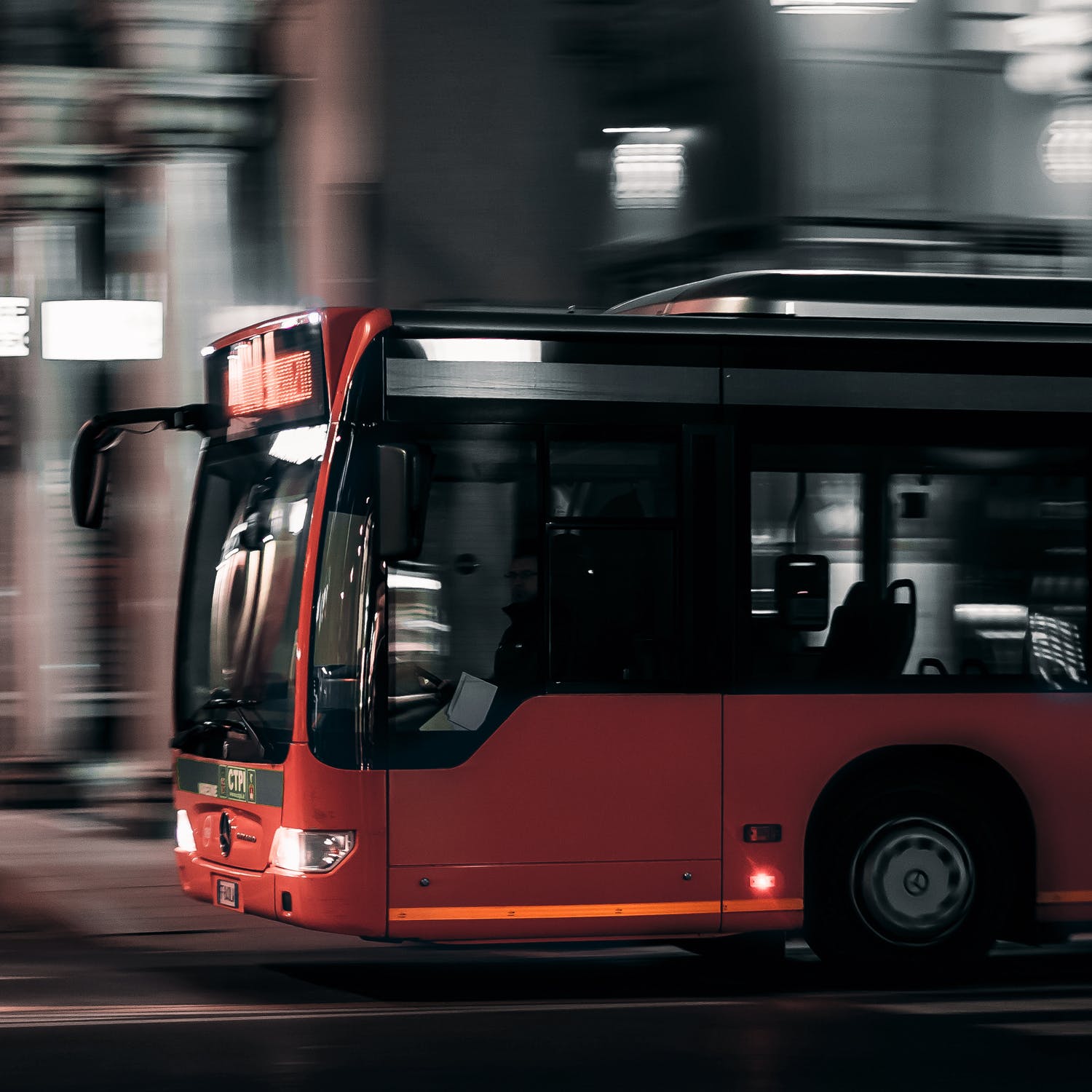
A suspension system of a bus can be modeled as below.
 |
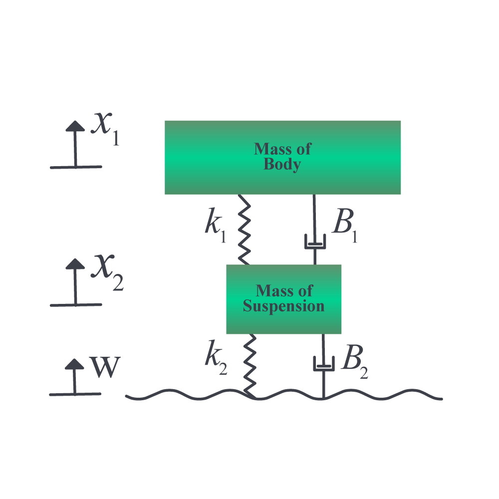 |
Figure 1: a) School bus b) A model of 1/4th of suspension system of a bus (Credit: Model and numbers from <http://www.monografias.com/trabajos-pdf/modeling-bus-suspension-transfer-function/modeling-bus-suspension-transfer-function.pdf>)
Only 1/4th of the bus is modeled. The differential equations that govern the above system can be derived (this is something you will do in your vibrations course) as
\[M_{1}\frac{d^{2}x_{1}}{dt^{2}} + B_{1}\left( \frac{dx_{1}}{{dt}} - \frac{dx_{2}}{{dt}} \right) + K_{1}\left( x_{1} - x_{2} \right) = 0\;\;\;\;\;\;\;\;\;\;\;\; (E3.1)\]
\[\begin{split} M_{2}\frac{d^{2}x_{2}}{dt^{2}} + B_{1}\left( \frac{dx_{2}}{{dt}} - \frac{dx_{1}}{{dt}} \right) &+ K_{1}\left( x_{2} - x_{1} \right) + B_{2}\left( \frac{dx_{2}}{{dt}} - \frac{{dw}}{{dt}} \right)\\ & \ \ \ \ \ \ + K_{2}\left( x_{2} - w \right) = 0\;\;\;\;\;\;\;\;\;\;\;\; (E3.2) \end{split}\]
\[x_{1}(0) = 0,x_{3}(0) = 0,x_{2}(0) = 0,x_{4}(0) = 0\]
where
\[M_{1} =\text{body mass}\]
\[M_{2} =\text{suspension mass}\]
\[K_{1} =\text{spring constant of the suspension system}\]
\[K_{2} =\text{spring constant of wheel and tire}\]
\[B_{1} =\text{damping constant of the suspension system}\]
\[B_{2} =\text{damping constant of wheel and tire}\]
\[x_{1} =\text{displacement of the body mass as a function of time}\]
\[x_{2} =\text{displacement of the suspension mass as a function of time}\]
\[w =\text{input profile of the road as a function of time}\]
The constants are given as
\[m_{1} = 2500\ \text{kg}\]
\[m_{2} = 320\ \text{kg}\]
\[k_{1} = 80000\ \text{N/m},\]
\[k_{2} = 500000\ \text{N/m},\]
\[B_{1} = 350\ \text{N-s/m},\]
\[B_{2} = 15020\ \text{N-s/m}\]
Reduce the simultaneous differential equations (E3.1) and (E3.2) to simultaneous first-order differential equations and put those in the state variable form complete with corresponding initial conditions.
Solution
Substituting the values of the constants in the two differential equations (1) and (2) gives the differential equations (3) and (4), respectively.
\[2500\frac{d^{2}x_{1}}{dt^{2}} + 350\left( \frac{dx_{1}}{{dt}} - \frac{dx_{2}}{{dt}} \right) + 80000\left( x_{1} - x_{2} \right) = 0\;\;\;\;\;\;\;\;\;\;\;\; (E3.3)\]
\[\begin{split} &320\frac{d^{2}x_{2}}{dt^{2}} + 350\left( \frac{dx_{2}}{{dt}} - \frac{dx_{1}}{{dt}} \right) + 80000\left( x_{2} - x_{1} \right) + 15020\left( \frac{dx_{2}}{{dt}} - \frac{{dw}}{{dt}} \right) +\\ & 500000(x_{2} - w) = 0\;\;\;\;\;\;\;\;\;\;\;\; (E3.4) \end{split}\]
Since \(w\) is an input, we take it to the right-hand side to show it as a forcing function and rewrite Equations (E3.4) as
\[\begin{split} &320\frac{d^{2}x_{2}}{dt^{2}} + 350\left( \frac{dx_{2}}{{dt}} - \frac{dx_{1}}{{dt}} \right) + 80000\left( x_{2} - x_{1} \right) + 15020\left( \frac{dx_{2}}{{dt}} \right) + 500000x_{2}\\ &=15020\frac{dw}{dt}+500000w\;\;\;\;\;\;\;\;\;\;\;\; (E3.5) \end{split}\]
Now let us start the process of reducing the 2 simultaneous differential equations (Equations (E3.3) and (E3.5)) to 4 simultaneous first-order ordinary differential equations.
Choose
\[\frac{dx_{1}}{{dt}} = x_{3},\;\;\;\;\;\;\;\;\;\;\;\; (E3.6)\]
\[\frac{dx_{2}}{{dt}} = x_{4},\;\;\;\;\;\;\;\;\;\;\;\; (E3.7)\]
then Equation (E3.3)
\[2500\frac{d^{2}x_{1}}{dt^{2}} + 350\left( \frac{dx_{1}}{{dt}} - \frac{dx_{2}}{{dt}} \right) + 80000\left( x_{1} - x_{2} \right) = 0\]
can be written as
\[2500\frac{dx_{3}}{{dt}} + 350\left( x_{3} - x_{4} \right) + 80000\left( x_{1} - x_{2} \right) = 0\]
\[2500\frac{dx_{3}}{{dt}} = - 350(x_{3} - x_{4}) - 80000(x_{1} - x_{2})\]
\[\begin{split} \frac{dx_{3}}{{dt}} &= - 0.14\left( x_{3} - x_{4} \right) - 32\left( x_{1} - x_{2} \right)\\ &= - 32x_{1} - 0.14x_{3} + 32x_{2} + 0.14x_{4}\;\;\;\;\;\;\;\;\;\;\;\; (E3.8)\end{split}\]
and Equation (E3.5)
\[\begin{split} &320\frac{d^{2}x_{2}}{dt^{2}} + 350\left( \frac{dx_{2}}{{dt}} - \frac{dx_{1}}{{dt}} \right) + 80000\left( x_{2} - x_{1} \right) + 15020\left( \frac{dx_{2}}{{dt}} \right) + 500000x_{2} \\ &= 15020\frac{{dw}}{{dt}} + 500000w \end{split}\]
can be written as
\[\begin{split} &320\frac{dx_{4}}{{dt}} + 350\left( x_{4} - x_{3} \right) + 80000\left( x_{2} - x_{1} \right) + 15020x_{4} + 500000x_{2}\\ &= 15020\frac{{dw}}{{dt}} + 500000w \end{split}\]
\[\begin{split} 320\frac{dx_{4}}{{dt}} = &- 350(x_{4} - x_{3}) - 80000(x_{2} - x_{1}) - 15020x_{4} - \\ & 500000x_{2} + 15020\frac{{dw}}{{dt}} + 500000w \end{split}\]
\[\begin{split} \frac{dx_{4}}{{dt}} &= - 1.09375\left( x_{4} - x_{3} \right) - 250\left( x_{2} - x_{1} \right) - 46.9375x_{4} - 1562.5x_{2}\\& \ \ \ \ \ \ \ \ \ \ + 46.9375\frac{{dw}}{{dt}} + 1562.5w\\ &= 250x_{1} + 1.09375x_{3} - 1812.5x_{2} - 48.03125x_{4}\\ &\ \ \ \ \ \ \ \ \ \ + 1562.5w + 46.9375\frac{{dw}}{{dt}}\ \ \ \ \ \ \ \ \ (E3.9) \end{split}\]
The 4 simultaneous first-order differential equations given by Equations (E3.6) thru (E3.9), complete with the corresponding initial condition, are
\[\begin{split} \frac{dx_{1}}{{dt}} &= x_{3}\\ &=f_1\left(t,x_1,x_2,x_3,x_4\right)\ \text{with } x_1\left(0\right)=0\;\;\;\;\;\;\;\;\;\;\;\; (E3.10) \end{split}\]
\[\begin{split} \frac{dx_{2}}{{dt}} &= x_{4}\\ &=f_2\left(t,x_1,x_2,x_3,x_4\right)\text{with }x_2\left(0\right)=0\;\;\;\;\;\;\;\;\;\;\;\; (E3.11) \end{split}\]
\[\begin{split} \frac{dx_{3}}{{dt}} &= - 32x_{1} + 32x_{2} - 0.14x_{3} + 0.14x_{4}\\ &=f_3\left(t,x_1,x_2,x_3,x_4\right)\text{with }x_3\left(0\right)=0\;\;\;\;\;\;\;\;\;\;\;\; (E3.12) \end{split}\]
\[\begin{split} \frac{dx_{4}}{{dt}} &= 250x_{1} - 1812.5x_{2} + 1.09375x_{3} - 48.03125x_{4} + 1562.5w + 46.9375\frac{{dw}}{{dt}}\\ &=f_4\left(t,x_1,x_2,x_3,x_4\right)\text{with }x_4\left(0\right)=0\;\;\;\;\;\;\;\;\;\;\;\; (E3.13) \end{split}\]
The profile of the road is given below.
Assuming that the bus is going at \(60 \ \text{mph}\), that is, approximately \(27 \ \text{m/s}\), it takes
\[\frac{6m}{27{m/s}} = 0.22\ \text{s}\]
to go through one period. So the frequency
\[\begin{split} f &= \frac{1}{0.22}\\ &= {4.545\ \ \text{Hz}}\end{split}\]
The angular frequency then is
\[\begin{split} \omega &=2 \times \pi \times4.545\\ &= 28.6\ \text{rad/s} \end{split}\]
giving
\[\begin{split} w &= 0.01\sin\left( {\omega t} \right)\\ &= 0.01\sin\left( 28.6t \right)\end{split}\]
and
\[\frac{{dw}}{{dt}} = 0.286\cos\left( 28.6t \right)\]
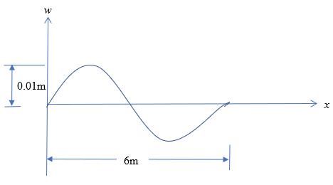
Figure 2: Periodic road profile
To put the differential equations given by Equations (E3.10)-(E3.13) in matrix form, we rewrite them as
\[\frac{dx_{1}}{{dt}} = x_{3} = 0x_{1} + 0x_{2} + 1x_{3} + 0x_{4},\ {x}_{1}\left( 0 \right) = 0\;\;\;\;\;\;\;\;\;\;\;\; (E3.14)\]
\[\frac{dx_{2}}{{dt}} = x_{4} = 0x_{1} + 0x_{2} + 0x_{3} + 1x_{4},\ {x}_{2}\left( 0 \right) = 0\;\;\;\;\;\;\;\;\;\;\;\; (E3.15)\]
\[\frac{dx_{3}}{{dt}} = - 32x_{1} + 32x_{2} - 0.14x_{3} + 0.14x_{4},\ x_{3}\left( 0 \right) = 0\;\;\;\;\;\;\;\;\;\;\;\; (E3.16)\]
\[\begin{split} \frac{dx_{4}}{{dt}} = &250x_{1} - 1812.5x_{2} + 1.09375x_{3} - 48.03125x_{4} + \\ &1562.5w + 46.9375\frac{{dw}}{{dt}},\ x_{4}\left( 0 \right) = 0\;\;\;\;\;\;\;\;\;\;\;\; (E3.17) \end{split}\]
In state variable matrix form, the differential equations are given by
\[\begin{split} \begin{bmatrix} \displaystyle \frac{dx_{1}}{{dt}} \\ \displaystyle \frac{dx_{2}}{{dt}} \\ \displaystyle \frac{dx_{3}}{{dt}} \\ \displaystyle \frac{dx_{4}}{{dt}} \\ \end{bmatrix} &= \begin{bmatrix} 0 & 0 & 1 & 0 \\ 0 & 0 & 0 & 1 \\ - 32 & 32 & - 0.14 & 0.14 \\ 250 & - 1812.5 & 1.09375 & - 48.03125 \\ \end{bmatrix}\begin{bmatrix} x_{1} \\ x_{2} \\ x_{3} \\ x_{4} \\ \end{bmatrix} \\ & \ \ \ \ \ \ \ \ \ \ \ \ \ \ \ \ \ \ \ \ \ \ \ \ \ \ \ \ \ \ \ \ \ \ \ \ \ \ + \begin{bmatrix} 0 \\ 0 \\ 0 \\ 1562.5w + 46.9375\displaystyle \frac{{dw}}{{dt}} \\ \end{bmatrix} \;\;\;\;\;\;\;\;\;\;\;\; (E3.18)\end{split}\]
where
\[w = 0.01\sin(28.6t) \;\;\;\;\;\;\;\;\;\;\;\; (E3.19)\]
and the corresponding initial conditions are
\[\begin{bmatrix} x_{1}(0) \\ x_{2}(0) \\ x_{3}(0) \\ x_{4}(0) \\ \end{bmatrix} = \begin{bmatrix} 0 \\ 0 \\ 0 \\ 0 \\ \end{bmatrix}\]
Can you identify the state vector, the state matrix, the input vector, and the initial conditions on the state vector?
State-space models is how numerical solvers expect you to enter the data. For example, the above state-space model would be entered as the following on MATLAB.
First, a function is defined where t is the independent variable, and x is the state-space vector. The names diffx and sysofeqn are the choice of the user. The arguments of the function are the independent variable t and the state vector x. Inside the function, [A] is the state-space matrix from Equation (E3.18), \(w\) is the forcing function from Equation (E3.19), [B] is the input vector.
function diffx=sysofeqn(t,x)
A=[0 0 1 0; …
0 0 0 1; …
-32 32 -0.14 0.14; …
250 -1812.5 1.09375 -48.03125];
w=0.01*sin(28.6*t);
dw=0.286*cos(28.6*t);
B=[0; 0; 0; 1652.5*w+46.9375*dw];
diffx=A*x+B;
end
How is the function used? Assume that you want the output between t=0 and 10. You can use that time span shown as tspan variable. Then the initial conditions of the state vector are entered. The ode45 routine is a combination of the Runge-Kutta 4th and 5th order methods to solve a system of first-order ordinary differential equations. The inputs of the ode45 routine are the system of equations, the span in which the output is requested, and the initial conditions.
tspan=[0 10];
initial_cond=[0;0;0;0];
[t,x]=ode45('sysofeqn',tspan,initial_cond);
figure (1)
plot(t,x(:,1))
A sample of the outputs is shown below with the values of the independent variable t, the state vector x, and the output of x(1) vs t.


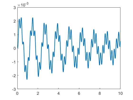
Figure 3: Output values and \(x_1\) vs. \(t\) for the bus-suspension problem.
Problem Set
(1). Reduce the following 2nd order ordinary differential equation to a set of first-order ordinary differential equations complete with initial conditions and in the form required to solve them numerically.
\[5\frac{d^{2}y}{dt^{2}} + 3\frac{dy}{dt} + 7y = e^{- t} + t^{2},\ y(0) = 6,\ \frac{dy}{dt}(0) = 11.\]
(2). Reduce the following coupled ordinary differential equations to a set of first-order ordinary differential equations complete with initial conditions and in the form required for solving them numerically.
\[10\frac{d^{2}x_{1}}{dt^{2}} - 15( - 2x_{1} + x_{2}) = 0,\]
\[20\frac{d^{2}x_{2}}{dt^{2}} - 15(x_{1} - 2x_{2}) = 0,\]
\[x_{1}(0) = 2,\ x_{2}(0) = 3,\ \frac{dx_{1}}{dt}(0) = 4,\ \frac{dx_{2}}{dt}(0) = 5.\]
(3). The acceleration of a spring-mass system is given by \((t > 0)\)
\[\frac{d^{2}x}{dt^{2}} + x = e^{- t}\]
where \(x\) is the displacement of the mass given in meters and \(t\) is the time given in seconds. The initial conditions are given as \(x(0) = 3\), \(\displaystyle \frac{dx}{dt}(0) = 2\).
a) What is the value of displacement, velocity, and acceleration at \(t = 0 +\) seconds.
b) Use Euler’s method to find the value of displacement, velocity, and acceleration at \(t = 0.5\) seconds. Use a step size of \(0.25\) seconds.
c) What is the exact value of displacement, velocity and acceleration at \(t = 0.5\) seconds.
Answer: \(a)\ 3,\ 2 ,\ -2\)
\(b)\ 3.8750,\ 0.81970,\ -3.2685\)
\(c)\ 3.6958,\ 0.69213,\ -3.0893\)
(4). The acceleration of a spring-mass system is given by
\[\frac{d^{2}x}{dt^{2}}\ + x = \ e^{- t}\]
where \(x\) is the displacement of the mass given in meters and \(t\) is the time given in seconds. The initial conditions are given as \(x(0) = 3\), \(\displaystyle \frac{dx}{dt}(0) = 2\). Use Runge Kutta 2nd order Ralston’s method to find the value of displacement, velocity, and acceleration at \(t = 0.5\) seconds. Use a step size of \(0.25\) seconds.
Answer: \(3.7067\ m,\ 0.67811\ m/s,\ -3.1001\ m/s^2\)
(5). Reduce the following ordinary differential equation to the state-space model form. Include the initial conditions in proper form as well.
\[4\frac{d^{2}y}{dt^{2}} + 9\frac{dy}{dt} + 12y = 3sin(7x),\ y(0) = 13,\ \frac{dy}{dt}(0) = 19.\]
(6). Reduce the following coupled ordinary differential equations to the state space model form. Include the initial conditions in proper form as well.
\[25\frac{d^{2}x_{1}}{dt^{2}} - 40( - 3x_{1} + x_{2}) = 3 cos(3t),\]
\[32\frac{d^{2}x_{2}}{dt^{2}} - 12x_{1} - 24x_{2} = 7e^{-3t},\]
\[x_{1}(0) = 23,\ x_{2}(0) = 17,\ \frac{dx_{1}}{dt}(0) = 37,\ \frac{dx_{2}}{dt}(0) = 29.\]