Chapter 08.03: Runge-Kutta 2nd-Order Method for Solving Ordinary Differential Equations
Learning Objectives
After successful completion of this lesson, you should be able to:
1) list the formulas of the Runge-Kutta 2nd order method for ordinary differential equations and know how to use them.
What is the Runge-Kutta 2nd order method?
The Runge-Kutta 2nd order method is a numerical technique used to solve an ordinary differential equation of the form
\[\frac{{dy}}{{dx}} = f\left( x,y \right),\ y\left( x_0 \right) = y_{0}\;\;\;\;\;\;\;\;\;\;\;\; (1)\]
Only first-order ordinary differential equations of the form of Equation (1) can be solved by using the Runge-Kutta 2nd order method. In other sections, we discuss how the Euler and Runge-Kutta methods are used to solve higher-order ordinary or coupled (simultaneous) ordinary differential equations.
How does one write a first-order ordinary differential equation in the above form?
Runge-Kutta 2nd order method
Euler’s method is given by
\[y_{i + 1} = y_{i} + f\left( x_{i},y_{i} \right)h\;\;\;\;\;\;\;\;\;\;\;\; (2)\]
where
\[y(x_0)=y_0\]
\[h = x_{i + 1} - x_{i}\]
To understand the Runge-Kutta 2nd order method, we need to first derive Euler’s method from the Taylor series.
\[\begin{split} y_{i + 1} &= y_{i} + \left. \ \frac{{dy}}{{dx}} \right|_{x_{i},y_{i}}\left( x_{i + 1} - x_{i} \right) + \frac{1}{2!}\left. \ \frac{d^{2}y}{dx^{2}} \right|_{x_{i},y_{i}}\left( x_{i + 1} - x_{i} \right)^{2}\\ &\ \ \ \ \ \ \ \ \ \ \ \ \ \ \ \ \ \ + \frac{1}{3!}\left. \ \frac{d^{3}y}{dx^{3}} \right|_{x_{i},y_{i}}\left( x_{i + 1} - x_{i} \right)^{3} + ... \end{split}\]
Since \(\displaystyle \frac{dy}{dx}=f(x,y)\)
\[\begin{split} y_{i+1} &= y_{i} + f(x_{i},y_{i})\left( x_{i + 1} - x_{i} \right) + \frac{1}{2!}f'(x_{i},y_{i})\left( x_{i + 1} - x_{i} \right)^{2}\\ &\ \ \ \ \ \ \ \ \ \ \ \ \ \ \ \ \ \ + \frac{1}{3!}f''(x_{i},y_{i})\left( x_{i + 1} - x_{i} \right)^{3} + ...\;\;\;\;\;\;\;\;\;\;\;\; (3) \end{split}\]
As you can see, the first two terms of the Taylor series in Equation (3)
\[y_{i + 1} = y_{i} + f\left( x_{i},y_{i} \right)h\]
represent Euler’s method and hence can be considered to be a Runge-Kutta 1st order method.
The true error in the approximation is given by
\[E_{t} = \frac{f^{\prime}\left( x_{i},y_{i} \right)}{2!}h^{2} + \frac{f^{\prime\prime}\left( x_{i},y_{i} \right)}{3!}h^{3} + ...\;\;\;\;\;\;\;\;\;\;\;\; (4)\]
So what would a 2nd order method formula look like? It would include one more term of the Taylor series as follows.
\[y_{i + 1} = y_{i} + f\left( x_{i},y_{i} \right)h + \frac{1}{2!}f^{\prime}\left( x_{i},y_{i} \right)h^{2}\;\;\;\;\;\;\;\;\;\;\;\; (5)\]
Let us take a generic example of a first-order ordinary differential equation
\[\frac{{dy}}{{dx}} = e^{- 2x} - 3y,y\left( 0 \right) = 5\]
\[f\left( x,y \right) = e^{- 2x} - 3y\]
Now since \(y\) is a function of \(x\),
\[\begin{split} f^{\prime}\left( x,y \right) &= \frac{\partial f\left( x,y \right)}{\partial x} + \frac{\partial f\left( x,y \right)}{\partial y}\frac{{dy}}{{dx}}\;\;\;\;\;\;\;\;\;\;\;\; (6)\\ &= \frac{\partial}{\partial x}\left( e^{- 2x} - 3y \right) + \frac{\partial}{\partial y}\left\lbrack \left( e^{- 2x} - 3y \right) \right\rbrack\left( e^{- 2x} - 3y \right)\\ &= - 2e^{- 2x} + ( - 3)\left( e^{- 2x} - 3y \right)\\ &= - 5e^{- 2x} + 9y \end{split}\]
The 2nd order formula for the above example would be
\[\begin{split} y_{i + 1} &= y_{i} + f\left( x_{i},y_{i} \right)h + \frac{1}{2!}f^{\prime}\left( x_{i},y_{i} \right)h^{2}\\ &= y_{i} + \left( e^{- 2x_{i}} - 3y_{i} \right)h + \frac{1}{2!}\left( - 5e^{- 2x_{i}} + 9y_{i} \right)h^{2} \end{split}\]
However, we already recognize the pitfall of having to find \(f^{\prime}\left( x,y \right)\) in the above method. What Runge and Kutta did was write the 2nd order method as
\[y_{i + 1} = y_{i} + \left( a_{1}k_{1} + a_{2}k_{2} \right)h\;\;\;\;\;\;\;\;\;\;\;\; (7)\]
where
\[k_{1} = f\left( x_{i},y_{i} \right)\;\;\;\;\;\;\;\;\;\;\;\; (8a)\]
\[k_{2} = f\left( x_{i} + p_{1}h,y_{i} + q_{11}k_{1}h \right)\;\;\;\;\;\;\;\;\;\;\;\; (8b)\]
This form allows one to take advantage of the 2nd order method without having to calculate \(f^{\prime}\left( x,y \right)\).
So how do we find the unknowns \(a_{1}\), \(a_{2}\), \(p_{1},\) and \(q_{11}\)? Without proof, equating Equation (5) and (7), gives three equations.
\[a_{1} + a_{2} = 1\;\;\;\;\;\;\;\;\;\;\;\; (9a)\]
\[a_{2}p_{1} = \frac{1}{2}\;\;\;\;\;\;\;\;\;\;\;\; (9b)\]
\[a_{2}q_{11} = \frac{1}{2}\;\;\;\;\;\;\;\;\;\;\;\; (9c)\]
Since we have 3 equations and 4 unknowns, we can assume the value of one of the unknowns. The other three are then determined from the three equations. Generally, the value of \(a_{2}\) is chosen to evaluate the other three constants. The three values used for \(a_{2}\) are \(\displaystyle \frac{1}{2}\), \(1\) and \(\displaystyle \frac{2}{3}\), and are known as Heun’s Method, the midpoint method, and Ralston’s method, respectively.
Heun’s Method
Here \(a_{2} = \displaystyle \frac{1}{2}\) is chosen, and from Equations (9a)-(9c),
\[a_{1}\ = \frac{1}{2}\]
\[p_{1}\ = 1\]
\[q_{11} = 1\]
resulting in
\[y_{i + 1} = y_{i} + \left( \frac{1}{2}k_{1} + \frac{1}{2}k_{2} \right)h\;\;\;\;\;\;\;\;\;\;\;\; (10)\]
where
\[k_{1} = f\left( x_{i},y_{i} \right)\;\;\;\;\;\;\;\;\;\;\;\; (11a)\]
\[k_{2} = f\left( x_{i} + h,y_{i} + k_{1}h \right)\;\;\;\;\;\;\;\;\;\;\;\; (11b)\]
This method is graphically explained in Figure 1.
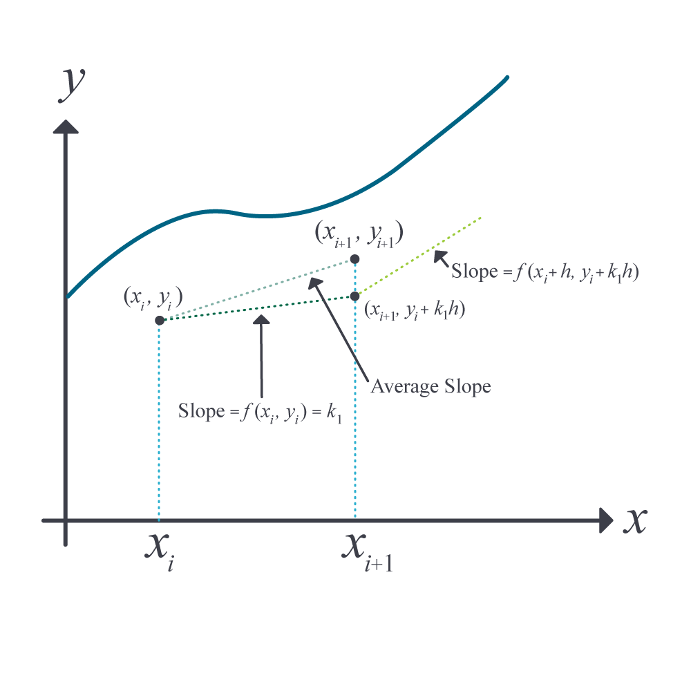
Figure 1 Runge-Kutta 2nd order method (Heun’s method).
Midpoint Method
Here \(a_{2} = 1\) is chosen, and from Equations (9a)-(9c),
\[a_{1} = 0\]
\[p_{1} = \frac{1}{2}\]
\[q_{11} = \frac{1}{2}\]
resulting in
\[y_{i + 1} = y_{i} + k_{2}h\;\;\;\;\;\;\;\;\;\;\;\; (12)\]
where
\[k_{1} = f\left( x_{i},y_{i} \right)\;\;\;\;\;\;\;\;\;\;\;\; (13a)\]
\[k_{2} = f\left( x_{i} + \frac{1}{2}h,y_{i} + \frac{1}{2}k_{1}h \right)\;\;\;\;\;\;\;\;\;\;\;\; (13b)\]
Ralston’s Method
Here \(a_{2} = \displaystyle\frac{2}{3}\) is chosen, and from Equations (9a)-(9c),
\[a_{1} = \frac{1}{3}\]
\[p_{1} = \frac{3}{4}\]
\[q_{11} = \frac{3}{4}\]
resulting in
\[y_{i + 1} = y_{i} + \left( \frac{1}{3}k_{1} + \frac{2}{3}k_{2} \right)h\;\;\;\;\;\;\;\;\;\;\;\;(14)\]
where
\[k_{1} = f\left( x_{i},y_{i} \right)\;\;\;\;\;\;\;\;\;\;\;\; (15a)\]
\[k_{2} = f\left( x_{i} + \frac{3}{4}h,y_{i} + \frac{3}{4}k_{1}h \right)\;\;\;\;\;\;\;\;\;\;\;\; (15b)\]
Learning Objectives
After successful completion of this lesson, you should be able to:
1) Use Runge 2nd order method to solve first-order ordinary differential equations.
Recap
In the previous lesson, we discussed the theory behind the Runge-Kutta 2nd order method of solving an ordinary differential equation of the form \(dy/dx=f(x,y)\) where \(y(x_0)=y_0\). In this lesson, we take an example of how to apply the algorithm of the Runge-Kutta 2nd order method.
Example 1
A ball at \(1200\ \text{K}\) is allowed to cool down in air at an ambient temperature of \(300\ \text{K}\). Assuming heat is lost only due to radiation, the differential equation for the temperature of the ball is given by
\[\frac{{d\theta }}{{dt}} = - 2.2067 \times {1}{0}^{{-12}}\ (\theta^{4} - 81 \times 10^{8})\]
where \(\theta\) is in K and \(t\) in seconds. Find the temperature at \(t = 480\) seconds using Runge-Kutta 2nd order method. Assume a step size of \(h = 240\) seconds.
Solution
\[\frac{{d\theta }}{{dt}} = - 2.2067 \times 10^{- 12}\left( \theta^{4} - 81 \times 10^{8} \right)\]
\[f\left( t,\theta \right) = - 2.2067 \times 10^{- 12}\left( \theta^{4} - 81 \times 10^{8} \right)\]
As per Heun’s method given in the previous lesson for an ordinary differential equation,
\[\frac{{d\theta }}{{dt}} = f(t,\theta)\]
Heun’s method formula is given by
\[\theta_{i + 1} = \theta_{i} + \left( \frac{1}{2}k_{1} + \frac{1}{2}k_{2} \right)h\]
\[k_{1} = f\left( t_{i},\theta_{i} \right)\]
\[k_{2} = f\left( t_{i} + h,\theta_{i} + k_{1}h \right)\]
For Step 1,
\[i = 0,\ t_{0} = 0,\ \theta_{0} = \theta(0) = 1200\ \text{K}\]
\[\begin{split} t_1&=t_0+h\\ &=0+240\\ &=240\ \text{s}\end{split}\]
\[\begin{split} k_{1} &= f\left( t_{0},\theta_{o} \right)\\ &= f\left( 0,1200 \right)\\ &= - 2.2067 \times 10^{- 12}\left( 1200^{4} - 81 \times 10^{8} \right)\\ &= - 4.5579 \end{split}\]
\[\begin{split} k_{2} &= f\left( t_{0} + h,\theta_{0} + k_{1}h \right)\\ &= f\left( 0 + 240,1200 + \left( - 4.5579 \right)240 \right)\\ &= f\left( 240,106.09 \right)\\ &= - 2.2067 \times 10^{- 12}\left( 106.09^{4} - 81 \times 10^{8} \right)\\ &= 0.017595 \end{split}\]
\[\begin{split} \theta_{1} &= \theta_{0} + \left( \frac{1}{2}k_{1} + \frac{1}{2}k_{2} \right)h\\ &= 1200 + \left( \frac{1}{2}\left( - 4.5579 \right) + \frac{1}{2}\left( 0.017595 \right) \right)240\\ &= 1200 + \left( - 2.2702 \right)240\\ &= 655.16\ \text{K}\\ &\approx \theta(240) \end{split}\]
For Step 2
\[i = 1,t_{1} = 240 \ \text{s},\theta_{1} = 655.16\ \text{K}\]
\[\begin{split} &=t_1+h\\ &=240+240\\ &=480\ \text{s}\end{split}\]
\[\begin{split} k_{1} &= f\left( t_{1},\theta_{1} \right)\\ &= f\left( 240,655.16 \right)\\ &= - 2.2067 \times 10^{- 12}\left( 655.16^{4} - 81 \times 10^{8} \right)\\ &= - 0.38869 \end{split}\]
\[\begin{split} k_{2} &= f\left( t_{1} + h,\theta_{1} + k_{1}h \right)\\ &= f\left( 240 + 240,655.16 + \left( - 0.38869 \right)240 \right)\\ &= f\left( 480,561.87 \right)\\ &= - 2.2067 \times 10^{- 12}\left( 561.87^{4} - 81 \times 10^{8} \right)\\ &= - 0.20206 \end{split}\]
\[\begin{split} \theta_{2} &= \theta_{1} + \left( \frac{1}{2}k_{1} + \frac{1}{2}k_{2} \right)h\\ &= 655.16 + \left( \frac{1}{2}\left( - 0.38869 \right) + \frac{1}{2}\left( - 0.20206 \right) \right)240\\ &= 655.16 + \left( - 0.29538 \right)240\\ &= 584.27\ \text{K}\\ &\approx \theta(480) \end{split}\]
The results from Heun’s method are compared with the exact results in Figure 1.
The exact solution of the ordinary differential equation is given by the solution of a nonlinear equation as
\[0.92593\ln\frac{\theta - 300}{\theta + 300} - 1.8519\tan^{- 1}\left( 0.0033333\theta \right) = - 0.22067 \times 10^{- 3}t - 2.9282\]
The solution to this nonlinear equation at \(t = 480\ \text{s}\) is
\[\theta(480) = 647.57\ \text{K}\]
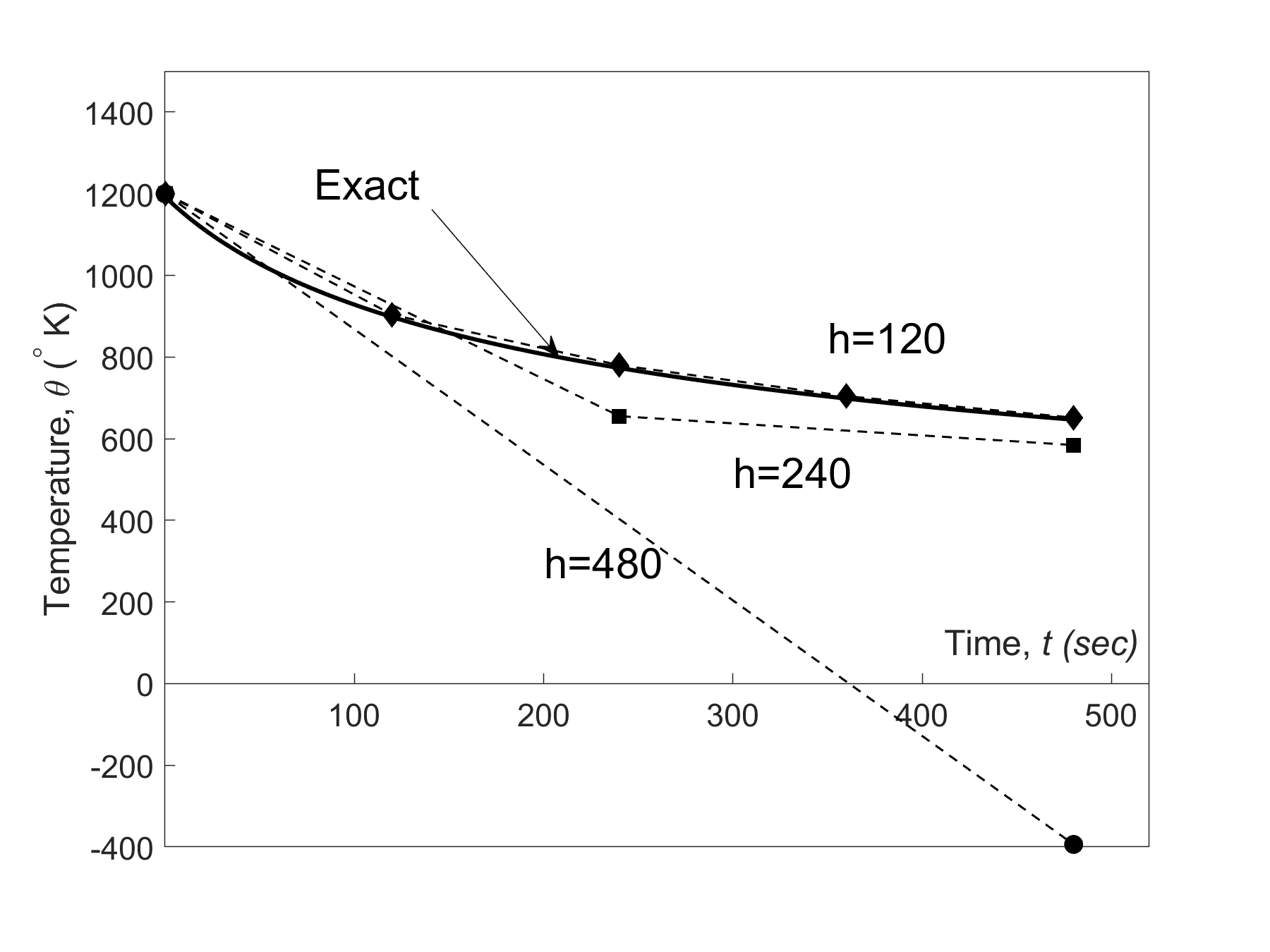
Figure 1 Heun’s method results for different step sizes.
Using a smaller step size would increase the accuracy of the result, as given in Table 1 and Figure 2 below.
Table 1 Effect of step size for Heun’s method
| \(Step\ size,\) \(h\) | \(\theta\left ( 480 \right)\) | \(E_{t}\) | \(\left| \epsilon_ {t} \right|\%\) |
|---|---|---|---|
\(480\) \(240\) \(120\) \(60\) \(30\) |
\(-393.87\) \(584.27\) \(651.35\) \(649.91\) \(648.21\) |
\(1041.4\) \(63.304\) \(-3.7762\) \(-2.3406\) \(-0.63219\) |
\(160.82\) \(9.7756\) \(0.58313\) \(0.36145\) \(0.097625\) |
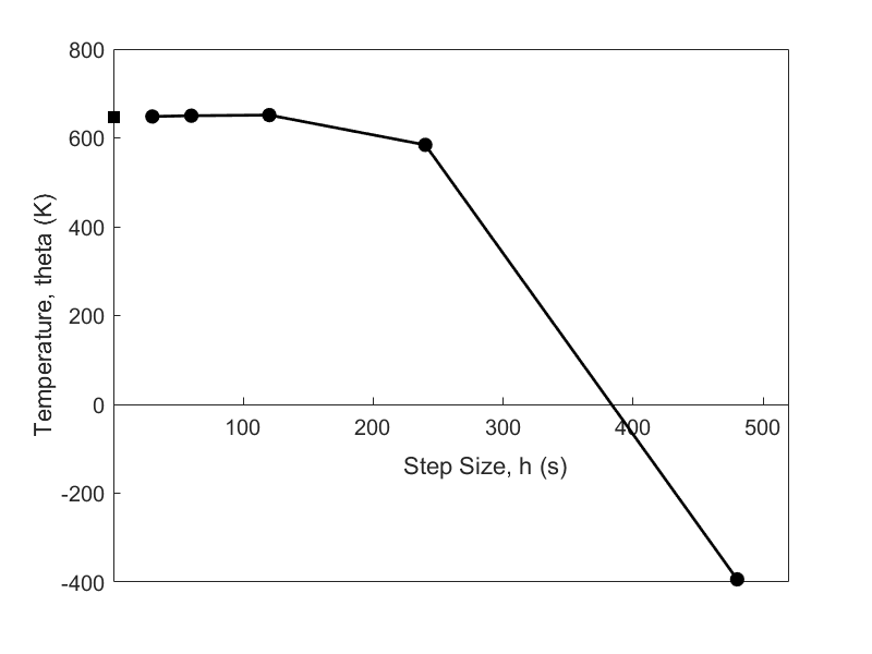
Figure 2 Effect of step size in Heun’s method.
In Table 2, Euler’s method and the Runge-Kutta 2nd order method results are shown as a function of step size,
Table 2 Comparison of Euler and the Runge-Kutta methods
| \(Step\ size,\) \(h\) | \(\theta(480)\) | |||
|---|---|---|---|---|
| \(Euler\) | \(Heun\) | \(Midpoint\) | \(Ralston\) | |
\(480\) \(240\) \(120\) \(60\) \(30\) |
\(-987.84\) \(110.32\) \(546.77\) \(614.97\) \(632.77\) |
\(-393.87\) \(584.27\) \(651.35\) \(649.91\) \(648.21\) |
\(1208.4\) \(976.87\) \(690.20\) \(654.85\) \(649.02\) |
\(449.78\) \(690.01\) \(667.71\) \(652.25\) \(648.61\) |
while in Figure 3, the comparison is shown over time.
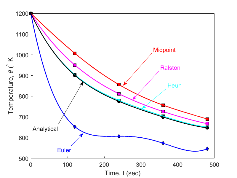
Figure 3 Comparison of Euler and Runge Kutta methods with exact results over time.
How do these three methods compare with results obtained if we found \(\mathbf{f^\prime (x,y)}\) directly?
Of course, we know that since we are including the first three terms in the series, if the solution is a polynomial of order two or less (that is, quadratic, linear, or constant), any of the three methods are exact. But for any other case, the results are going to be different.
Let us take the example of showing the difference in results.
\[\frac{{dy}}{{dx}} = e^{- 2x} - 3y,y\left( 0 \right) = 5.\]
If we directly find \(f^{\prime}\left( x,y \right)\), the first three terms of the Taylor series gives
\[y_{i + 1} = y_{i} + f\left( x_{i},y_{i} \right)h + \frac{1}{2!}f^{\prime}\left( x_{i},y_{i} \right)h^{2}\]
where
\[f\left( x,y \right) = e^{- 2x} - 3y\]
\[f^{\prime}\left( x,y \right) = - 5e^{- 2x} + 9y\]
For a step size of \(h = 0.2\), using Heun’s method, we find
\[y\left( 0.6 \right) = 1.0930\]
The exact solution
\[y\left( x \right) = e^{- 2x} + 4e^{- 3x}\]
gives
\[\begin{split} y\left( 0.6 \right) &= e^{- 2\left( 0.6 \right)} + 4e^{- 3\left( 0.6 \right)}\\ &= 0.96239 \end{split}\]
Then the absolute relative true error is
\[\begin{split} \left| \epsilon_{t} \right| &= \left| \frac{0.96239 - 1.0930}{0.96239} \right| \times 100\\ &= 13.571\% \end{split}\]
For the same problem, the results from Euler’s method and the three Runge-Kutta methods are given in Table 3.
Table 3 Comparison of Euler’s and Runge-Kutta 2nd order methods
| \(Exact\) | \(Euler\) | \(Direct\ 2nd\) | \(Heun\) | \(Midpoint\) | \(Ralston\) | |
|---|---|---|---|---|---|---|
| \(y(0.6)\) | \(0.96239\) | \(0.4955\) | \(1.0930\) | \(1.1012\) | \(1.0974\) | \(1.0994\) |
| \(\left| \epsilon_{t} \right|\) % | \(48.514\) | \(13.571\) | \(14.423\) | \(14.029\) | \(14.236\) |
Learning Objectives
After successful completion of this lesson, you should be able to:
1) derive the Runge-Kutta 2nd order method for the first-order ordinary differential equation.
How do we get the 2nd order Runge-Kutta method equations?
We wrote the 2nd order Runge-Kutta equations without proof to solve
\[\frac{{dy}}{{dx}} = f\left( x,y \right),\ y\left( 0 \right) = y_{0}\;\;\;\;\;\;\;\;\;\;\;\; (1)\]
as
\[y_{i + 1} = y_{i} + \left( a_{1}k_{1} + a_{2}k_{2} \right)h \;\;\;\;\;\;\;\;\;\;\;\; (2)\]
where
\[k_{1} = f\left( x_{i},y_{i} \right)\;\;\;\;\;\;\;\;\;\;\;\; (3a)\]
\[k_{2} = f\left( x_{i} + p_{1}h,y_{i} + q_{11}k_{1}h \right)\;\;\;\;\;\;\;\;\;\;\;\; (3b)\]
and
\[a_{1} + a_{2} = 1\;\;\;\;\;\;\;\;\;\;\;\; (4a)\]
\[a_{2}p_{2} = \frac{1}{2}\;\;\;\;\;\;\;\;\;\;\;\; (4b)\]
\[a_{2}q_{11} = \frac{1}{2}\;\;\;\;\;\;\;\;\;\;\;\; (4c)\]
The advantage of using 2nd order Runge-Kutta method equations is based on not having to find the derivative of \(f\left( x,y \right)\) symbolically in the ordinary differential equation
So how do we get the above three Equations ((A.4))4a)-(4c)? The question is answered below.
Writing out the first three terms of the Taylor series are
\[y_{i + 1} = y_{i} + \left. \ \frac{{dy}}{{dx}} \right|_{x_{i}y_{i}}h + \left. \ \frac{1}{2!}\frac{d^{2}y}{dx^{2}} \right|_{x_{i}y_{i}}h^{2} + O\left( h^{3} \right)\;\;\;\;\;\;\;\;\;\;\;\; (5)\]
where
\[h = x_{i + 1} - x_{i}\]
Since
\[\frac{{dy}}{{dx}} = f\left( x,y \right)\]
we can rewrite the Taylor series as
\[y_{i + 1} = y_{i} + f\left( x_{i},y_{i} \right)h + \frac{1}{2!}f^{\prime}\left( x_{i},y_{i} \right)h^{2} + O\left( h^{3} \right)\;\;\;\;\;\;\;\;\;\;\;\; (6)\]
Now
\[f^{\prime}\left( x,y \right) = \frac{\partial f\left( x,y \right)}{\partial x} + \frac{\partial f\left( x,y \right)}{\partial y}\frac{{dy}}{{dx}}.\;\;\;\;\;\;\;\;\;\;\;\; (7)\]
Hence
\[\begin{split} y_{i + 1} &= y_{i} + f\left( x_{i},y_{i} \right)h + \frac{1}{2!}\left( \left. \ \frac{\partial f}{\partial x} \right|_{x_{i},y_{i}} + \left. \ \frac{\partial f}{\partial y} \right|_{x_{i},y_{i}} \times \left. \ \frac{{dy}}{{dx}} \right|_{x_{i},y_{i}} \right)h^{2} + O\left( h^{3} \right)\\ &= y_{i} + f\left( x_{i},y_{i} \right)h + \frac{1}{2}\left. \ \frac{\partial f}{\partial x} \right|_{x_{i},y_{i}}h^{2} + \frac{1}{2}\left. \ \frac{\partial f}{\partial y} \right|_{x_{i},y_{i}}f\left( x_{i},y_{i} \right)h^{2} + O\left( h^{3} \right)\;\;\;\;\;\;\;\;\;\;\;\; (8) \end{split}\]
Now the term used in the Runge-Kutta 2nd order method for \(k_{2}\) can be written as a Taylor series of two variables with the first three terms as
\[\begin{split} k_{2} &= f\left( x_{i} + p_{1}h,y_{i} + q_{11}k_{1}h \right)\\ &= f\left( x_{i},y_{i} \right) + p_{1}h\left. \ \frac{\partial f}{\partial x} \right|_{x_{i},y_{i}} + q_{11}k_{1}h\left. \ \frac{\partial f}{\partial y} \right|_{x_{i},y_{i}} + O\left( h^{2} \right)\;\;\;\;\;\;\;\;\;\;\;\; (9) \end{split}\]
Hence
\[\begin{split} y_{i + 1} &= y_{i} + \left( a_{1}k_{1} + a_{2}k_{2} \right)h\\ &= y_{i} + \left( a_{1}f\left( x_{i},y_{i} \right) + a_{2}\left\{ f\left( x_{i},y_{i} \right) + p_{1}h\left. \ \frac{\partial f}{\partial x} \right|_{x_{i},y_{i}} + q_{11}k_{1}h\left. \ \frac{\partial f}{\partial y} \right|_{x_{i},y_{i}} + O\left( h^{2} \right) \right\} \right)h\\ &= y_{i} + \left( a_{1} + a_{2} \right)hf\left( x_{i},y_{i} \right) + a_{2}p_{1}h^{2}\left. \ \frac{\partial f}{\partial x} \right|_{x_{i},y_{i}} + a_{2}q_{11}f\left( x_{i},y_{i} \right)h^{2}\left. \ \frac{\partial f}{\partial y} \right|_{x_{i},y_{i}} + O\left( h^{3} \right)\;\;\;\;\;\;\;\;\;\;\;\; (10) \end{split}\]
Equating the terms in Equation (8) and Equation (10), we get
\[a_{1} + a_{2} = 1\]
\[a_{2}p_{1} = \frac{1}{2}\]
\[a_{2}q_{11} = \frac{1}{2}\]
Multiple Choice Test
(1). To solve the ordinary differential equation
\[3\frac{{dy}}{{dx}} + xy^{2} = \sin x,\ y\left( 0 \right) = 5\]
by the Runge-Kutta 2nd order method, you need to rewrite the equation as
(A) \(\displaystyle \frac{{dy}}{{dx}} = \sin x - xy^{2},\ y\left( 0 \right) = 5\)
(B) \(\displaystyle \frac{{dy}}{{dx}} = \frac{1}{3}\left( \sin x - xy^{2} \right),\ y\left( 0 \right) = 5\)
(C) \(\displaystyle \frac{{dy}}{{dx}} = \frac{1}{3}\left( - \cos x - \frac{xy^{3}}{3} \right),\ y\left( 0 \right) = 5\)
(D) \(\displaystyle \frac{{dy}}{{dx}} = \frac{1}{3}\sin x,\ y\left( 0 \right) = 5\)
(2). Given
\[3\frac{{dy}}{{dx}} + 5y^{2} = \sin x,\ y\left( 0.3 \right) = 5\]
and using a step size of \(h = 0.3\), the value of \(y\left( 0.9 \right)\) using the Runge-Kutta 2nd order Heun’s method is most nearly
(A) \(-4297.4\)
(B) \(-4936.7\)
(C) \(-0.21336\times 10^{14}\)
(D) \(-0.24489\times 10^{14}\)
(3). Given
\[3\frac{{dy}}{{dx}} + 5\sqrt{y} = e^{0.1x},\ y\left( 0.3 \right) = 5\]
and using a step size of \(h = 0.3\), the best estimate of \(\displaystyle \frac{{dy}}{{dx}}\left( 0.9 \right)\) using the Runge-Kutta 2nd order midpoint method most nearly is
(A) \(-2.2473\)
(B) \(-2.2543\)
(C) \(-2.6188\)
(D) \(-3.2045\)
(4). The velocity (m/s) of a body is given as a function of time (seconds) by
\[v\left( t \right) = 200\ln\left( 1 + t \right) - t,\ t \geq 0\]
Using the Runge-Kutta 2nd order Ralston method with a step size of \(5\) seconds, the distance in meters traveled by the body from \(t = 2\) to \(t = 12\) seconds is estimated most nearly as
(A) \(3904.9\)
(B) \(3939.7\)
(C) \(6556.3\)
(D) \(39397\)
(5). The Runge-Kutta 2nd order method can be derived by using the first three terms of the Taylor series of writing the value of \(y_{i + 1}\) (that is the value of \(y\)at \(x_{i + 1}\)) in terms of \(y_{i}\) (that is the value of \(y\) at \(x_{i}\)) and all the derivatives of \(y\)at \(x_{i}\). If \(h = x_{i + 1} - x_{i}\), the explicit expression for \(y_{i + 1}\) if the first three terms of the Taylor series are chosen for solving the ordinary differential equation
\[\frac{{dy}}{{dx}} + 5y = 3e^{- 2x},y\left( 0 \right) = 7\]
would be
(A) \(\displaystyle y_{i + 1} = y_{i} + \left( 3e^{- 2x_{i}} - 5y_{i} \right)h + 5\frac{h^{2}}{2}\)
(B) \(\displaystyle y_{i + 1} = y_{i} + \left( 3e^{- 2x_{i}} - 5y_{i} \right)h + \left( - 21e^{- 2x_{i}} + 25y_{i} \right)\frac{h^{2}}{2}\)
(C) \(\displaystyle y_{i + 1} = y_{i} + \left( 3e^{- 2x_{i}} - 5y_{i} \right)h + \left( - 6e^{- 2x_{i}} \right)\frac{h^{2}}{2}\)
(D) \(\displaystyle y_{i + 1} = y_{i} + \left( 3e^{- 2x_{i}} - 5y_{i} \right)h + \left( - 6e^{- 2x_{i}} + 5 \right)\frac{h^{2}}{2}\)
(6). A spherical ball is taken out of a furnace at \(1200\ \text{K}\) and is allowed to cool in air. You are given the following
\[\text{radius of ball} = 2\ \text{cm}\]
\[\text{specific heat of ball} = 420\ \text{J/kg} \cdot \text{K}\]
\[\text{density of ball} = 7800\ \text{kg/m}^{3}\]
\[\text{convection coefficient} = 350\ \text{J/s} \cdot \text{m}^{2} \cdot \text{K}\]
\[\text{ambient temperature} = 300\text{ K}\]
The ordinary differential equation that is given for the temperature \(\theta\) of the ball is
\[\frac{{d\theta}}{{dt}} = - 2.20673 \times 10^{- 13}\left( \theta^{4} - 81 \times 10^{8} \right)\]
if only radiation is accounted for. If convection is accounted for in addition to radiation, the ordinary differential equation is
(A) \(\displaystyle \frac{{d\theta}}{{dt}} = - 2.20673 \times 10^{- 13}\left( \theta^{4} - 81 \times 10^{8} \right) - 1.6026 \times 10^{- 2}\left( \theta - 300 \right), \theta(0)=1200\ \text{K}\)
(B) \(\displaystyle \frac{{d\theta}}{{dt}} = - 2.20673 \times 10^{- 13}\left( \theta^{4} - 81 \times 10^{8} \right) - 4.3982 \times 10^{- 2}\left( \theta - 300 \right), \theta(0)=1200\ \text{K}\)
(C) \(\displaystyle \frac{{d\theta}}{{dt}} = - 1.6026 \times 10^{- 2}\left( \theta - 300 \right), \theta(0)=1200\ \text{K}\)
(D) \(\displaystyle \frac{{d\theta}}{{dt}} = - 4.3982 \times 10^{- 2}\left( \theta - 300 \right), \theta(0)=1200\ \text{K}\)
For complete solution, go to
http://nm.mathforcollege.com/mcquizzes/08ode/quiz_08ode_runge2nd_solution.pdf
Problem Set
(1). For the ordinary differential equation
\[2\frac{dy}{dx} + 3 xy = e^{- 1.5x},y(0) = 5\]
use a step size of \(h = 2\) and Runge-Kutta 2nd order Ralston’s method to find \(y(6)\).
Answer: \(y(6)\approx-23684\)
(2). For the ordinary differential equation
\[2\frac{dy}{dx} + 3 y = e^{- 1.5x},y(0) = 5\]
a) use Runge-Kutta 2nd order midpoint method to find \(y(2.5)\) using \(h = 1.25\),
b) use Runge-Kutta 2nd order midpoint method to find \(\displaystyle \frac{{dy}}{{dx}}\ (2.5)\) using \(h = 1.25\),
c) true value of \(y(2.5)\),
d) absolute relative true error for part (a),
e) true error of \(\displaystyle \frac{dy}{dx}\ (2.5),\)
f) absolute relative true error for part (b).
Answer: \(a)\ y\left(2.5\right)\approx3.5433\)
\(b)\ -5.3031\)
\(c)\ 0.14699\)
\(d)\ 2310.6\%\)
\(e)\ -0.20872\)
\(f)\ 2440.8\%\)
(3). Find the approximate value of the integral \(\displaystyle \int_{3}^{8}{2e^{0.6x}dx}\) using Runge-Kutta 2nd order Heun’s method.
a) Use \(h = 2.5\) and compare the value with the exact value.
b) Use \(h = 1.25\) and compare the value with the exact value.
Answer: \(a)\ 454.46,\ 18.083\%\)
\(b)\ 402.74,\ 4.6441\%\)
(4). From problem (3a), is the value obtained using Heun’s Runge-Kutta 2nd order method same as 2-segment LRAM (Left Endpoint Rectangular Approximation), or 2-segment MRAM (Midpoint Rectangular Approximation), or 2-segment RRAM (Right Endpoint Rectangular Approximation) method of integration or composite trapezoidal rule with 2 segments? Explain.
Answer: \(454.46\), MRAM
(5). A water tank with a hole at the top and a circular hole at the bottom is shown in the figure.
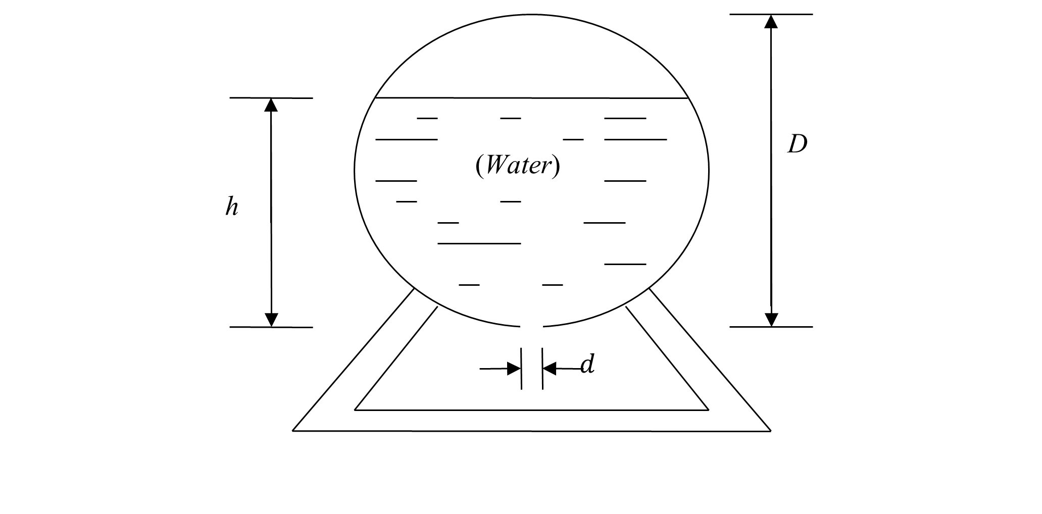
Given
\[\text{Diameter of the tank,}\ D = 6\ \text{m}\]
\[\text{Initial height of the water,}\ h = 5\ \text{m}\]
\[\text{Diameter of the hole,}\ d = 4.95\ \text{cm}\]
The flow rate \(\dot{Q}\) of water through the bottom hole, is given by
\[\dot{Q} = -{Av},\]
where
\[A =\text{cross-sectional area of the hole,}\]
\[v =\text{velocity of the water flowing through the hole.}\]
Since
\[v = \sqrt{2gh}\]
where
\[h =\text{height of the water from the bottom of the tank,}\]
\[g = \text{acceleration due to gravity.}\]
From this, we get
\[\dot{Q} = - A\sqrt{2gh}\]
Also, since the volume \(V\) of the water at height \(h\) is given by
\[V = \frac{1}{3}\pi h^{2}\left( \frac{3D}{2} - h \right)\]
where
\[\frac{dV}{dt} = \left( \pi hD - \pi h^{2} \right)\frac{dh}{dt}\]
Since
\[\dot{Q} = \frac{dV}{dt}\]
\[\left( \pi hD - \pi h^{2} \right)\frac{dh}{dt} = - A\sqrt{2gh}\]
\[\left( \pi hD - \pi h^{2} \right)\frac{dh}{dt} = - \frac{\pi d^{2}}{4}\sqrt{2gh}\]
\[\frac{dh}{dt} = - \frac{d^{2}\sqrt{2gh}}{4\left( hD - h^{2} \right)}\]
a) Use Runge-Kutta 2nd order Heun’s method with a step size of 10 minutes to find the height of water at \(t = 50\) minutes.
b) Based on the results from part (a), estimate the time when the height of the water is \(4\) m.
c) Compare the results of part(a) and part (b) with the exact values.
Answer: \(a)\ 2.9282\ \text{m}\)
\(b)\ 19.248\ \text{min}\)
\(c)\) part (a) \(h=2.9371\ \text{m},\ 0.303\%\)
part(b) \(t=19.41\ \text{min},\ 0.835\%\)
(6). For a spherical ball taken out of furnace at 2500 K that loses heat due to radiation and convection, the following is given.
\[\text{Radius of ball,}\ r = 1.0\ \text{cm},\]
\[\text{Density of the ball,}\ \rho = 3000\ \text{kg/m}^{3},\]
\[\text{Specific heat,}\ C = 1000\ \text{J}/(\text{kg} \cdot \text{K}),\]
\[\text{Emittance,}\ \in = 0.5,\]
\[\text{Stefan-Boltzmann Constant,}\ \sigma = 5.67 \times 10^{- 8}\ \text{J}/(\text{s} \cdot \text{m}^{2} \cdot \text{K}^{4}),\]
\[\text{Convective cooling coefficient,}\ h = 500\ \text{J/}(\text{s} \cdot \text{m}^{2} \cdot \text{K}),\]
\[\text{Initial temperature of the ball,}\ \theta(0) = 2500\ \text{K},\]
\[\text{Ambient temperature,}\ \theta_{a} = 300\ \text{K},\]
the ordinary differential equation that governs the temperature of the ball is given by
\[\frac{{d\theta}}{{dt}} = - 2.8349 \times 10^{- 12}(\theta^{4} - 81 \times 10^{8}) - 0.05(\theta - 300).\]
Hint: The above formula was calculated by using the knowledge that
\[\text{Rate of heat lost due to radiation}\ = A \in \sigma(\theta^{4} - \theta_{a}^{4})\]
\[\text{Rate of heat lost due to convection}\ = hA(\theta - \theta_{a})\]
\[\text{Heat stored}\ = mc\theta\]
where
\[A =\text{surface area of the ball,}\]
\[m =\text{mass of the ball.}\]
a) What are following at \(t = 0\ \text{s}\)?
temperature,
rate of change of temperature,
rate of heat loss due to radiation,
rate of heat loss due to convection,
rate of heat stored,
b) Find the following at \(t = 10\ \text{s}\) using Runge Kutta 2nd order Ralston’s method and a step size of \(h = 2.5\).
temperature,
rate of change of temperature,
rate of heat loss due to radiation,
rate of heat loss due to convection,
rate of heat stored,
c) Can either convection or radiation be neglected if we are interested in finding the temperature profile between \(0\) and \(10\ \text{s}\)? Base your answer on quantitative reasoning.
d) Find the time when the temperature will be \(2000\ \text{K}\) using Ralston’s method and a step size of \(h = 2.5\ \text{s}\).
Answer:
\(a)\ 2500\ \text{K},\ -220.72\ \text{K/s},\ 1391.3\ \text{W},\ 1382.3\ \text{W},\ -2773.6\ \text{W}\)
\(b)\ 1381.9\ \text{K},\ -64.41\ \text{K/s},\ 129.63\ \text{W},\ 679.78\ \text{W},\ -809.41\ \text{W}\)
\(c)\) Neither as rate of heat lost due to convection and radiation is of
same order.
\(d)\ 3.1591\ \text{s}\)