Chapter 06.00: Physical Problem for Regression
Summary
A student wants to pick the best mousetrap out of many for use in a mousetrap car. To do so, one requires to regress the torsion in the mousetrap spring to the angle through which it is opened.
Modeling
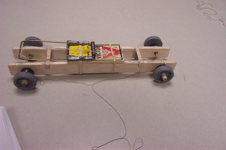
Figure 1 Mousetrap car.
In the Summer of 2003, a high school student worked with me to study the physics of a mousetrap car to build the car that would go the fastest and/or the farthest.
So what is a mousetrap car?
A mousetrap car (Figure 1) is a vehicle that is powered by the energy stored in the spring of a mousetrap. One of the basic ways most mousetrap vehicles are set into motion is by connecting the lever of the mousetrap bar through a string to the car’s axle. As the mousetrap lever is released, the tension that was built up in the spring is released, and the car sets into motion.
So to get the car to go the farthest and fastest, we need to store as much potential energy in the mousetrap spring. Since there is no specification on the mousetrap other than using a certain brand, we could use a mousetrap with the largest spring constant as that would translate to the largest potential energy stored.
Therefore, we bought several mousetrap springs and conducted a simple experiment to determine the spring constant of the mousetrap spring. These values of the spring constant would then allow us to find the potential energy stored in the mousetraps.
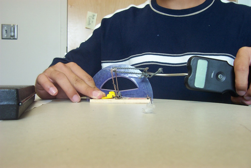
Figure 2 Experimental setup to measure the spring constant.
To find the spring constant of the mousetrap spring, we conducted the following experiment. We pulled the end of the mousetrap lever by a force probe (a fishhook) and measured the angle through which it is pulled by a protractor (Figure 2). We pulled on the end of the spring via a string so that the force on the lever is applied at a right angle to the lever. This way, the torque applied is simply the product of the force, as measured by the fishhook (Figure 3) and the length of the lever arm.
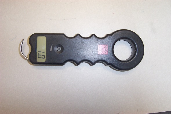
Figure 3 Force probe designed to measure the amount of force an object contains.
We measured the force needed to pull the lever for several different angles. The data for one of the mousetraps is given in Table 1.
The relationship between the torque applied and the angle of the rotation of the spring rotation is assumed to be a straight line
\[T = k_{0} + k_{1}{\theta}\;\;\;\;\;\;\;\;\;\;\;\; (1)\]
where
\[T = \text{Torque}\ \text{(N-m)}\]
\[\theta = \text{Angle through which the spring is rotated}\]
Table 1 Force vs. angle of lever rotation (Mousetrap #1).
| Angle (degrees) | Force (lbs) |
|---|---|
| \(40\) | \(0.9\) |
| \(55\) | \(1.0\) |
| \(65\) | \(1.1\) |
| \(90\) | \(1.2\) |
| \(110\) | \(1.5\) |
The data in Table 1 is converted to the SI system of units, and the torque is calculated using the measured lever moment arm of \(47\ \text{mm}\), that is
\[T = FL\;\;\;\;\;\;\;\;\;\;\;\; (2)\]
where,
\[T =\text{ Torque} \ \text{(N-m)}\]
\[F =\text{Force applied}\ \text{(N)}\]
\[L =\text{ Moment arm}\ \text{(m)}\]
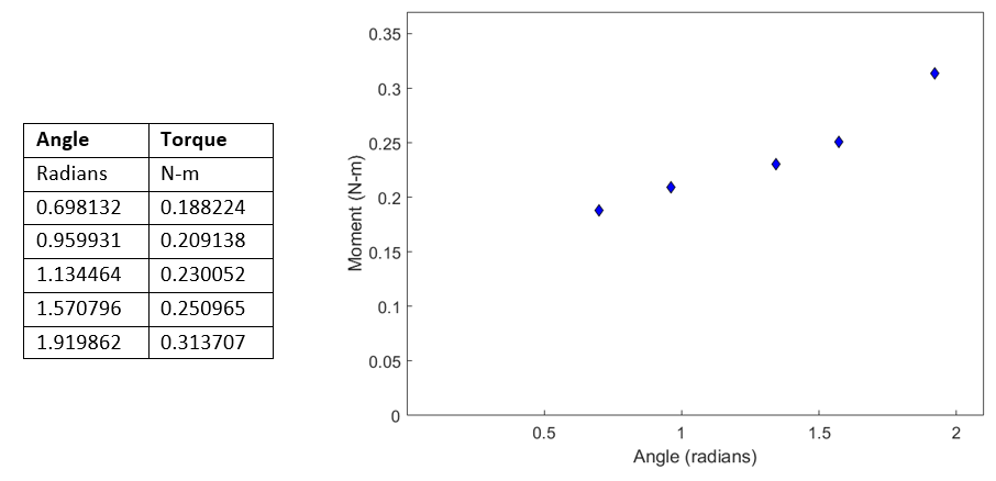
Figure 4 Data and plot of torque vs angle of rotation.
Other mousetrap springs were tested accordingly, and the data is given in Tables 2 and 3.
From these tables, we can find the \(T = k_{0} + k_{1}{\theta}\) relationship for each of three mousetraps. The potential energy, \(U\) stored in the spring would be given by
\[\begin{split} U &= \int_{\theta_{{low}}}^{\theta_{high}}T{d\theta}\\ &= \int_{\theta_{{low}}}^{\theta_{high}}(k_{0} + k_{1}\ \theta)d\theta \end{split}\]
Knowing that in our case, \(\theta_{{low}} = 0\) and \(\theta_{high} = \pi\), the maximum potential energy stored
\[\begin{split} U_{\max} &= \int_{0}^{\pi}(k_{0} + k_{1}\ \theta)d\theta\\ &= k_{0}\pi + k_{1}\frac{\pi^{2}}{2} \end{split}\;\;\;\;\;\;\;\;\;\;\;\; (3)\]
Table 2 Force vs. angle of lever rotation (Mousetrap #2).
| Angle (degrees) | Force (lbs) |
|---|---|
| \(38\) | \(0.9\) |
| \(58\) | \(1.0\) |
| \(65\) | \(1.1\) |
| \(90\) | \(1.2\) |
| \(120\) | \(1.6\) |
Table 3 Force vs. angle of lever rotation (Mousetrap #3).
| Angle (degrees) | Force (lbs) |
|---|---|
| \(40\) | \(0.9\) |
| \(57\) | \(1.0\) |
| \(65\) | \(1.1\) |
| \(90\) | \(1.2\) |
| \(135\) | \(1.7\) |
Questions
(1) Find the constants of the regression model for the spring for the three cases (Tables 1, 2, and 3).
(2) Based on maximum potential energy stored, which of the three springs would you choose?
Modeling
Chemical bonds have specific frequencies at which they will vibrate. These frequencies depend on the length of the bonds and the mass of the atoms at either end of bonds. Hence, vibrations of a molecule can be studied by shining infrared light onto the surface of the molecule. If one end of the molecular bond has a different charge from the other end (dipole moment), then the molecule can absorb infrared spectrum. However, this absorption occurs only at a certain fixed frequencies characteristic of the molecule and its component parts. Thus, an infrared light reflected from the surface of the bond will show absorption peaks characteristic of the molecule. This forms the basis of Infrared Spectroscopy (IRS).
To measure a sample, infrared light at a specific frequency is beamed onto the sample and the amount of energy absorbed is recorded. A chart is built up when this is repeated for several other frequencies. By examining the chart, one experienced in the art can identify the substance.
Fourier Transform Infrared Spectroscopy is a measurement technique for collecting infrared spectra and analyzing it. The wavenumber is the inverse of frequency while absorbance is proportional to the energy of the infrared light absorbed.
Table 1gives the FT-IR (Fourier Transform Infra Red) data of a 1:1 (by weight) mixture of ethylene carbonate (EC) and dimethyl carbonate (DMC). One would like to develop an equation which relates the absorbance as a function of wave number.
Table 1 Absorbance as a function of wavenumber
| Wavenumber | Absorbance |
|---|---|
| \(cm^{-1}\) | (arbitrary unit) |
| \(804.184\) | \(0.1591\) |
| \(808.041\) | \(0.1447\) |
| \(815.755\) | \(0.1045\) |
| \(821.540\) | \(0.0731\) |
| \(827.326\) | \(0.0439\) |
| \(829.254\) | \(0.0357\) |
| \(831.183\) | \(0.0285\) |
| \(833.111\) | \(0.0226\) |
| \(835.040\) | \(0.0178\) |
| \(836.968\) | \(0.0140\) |
| \(838.897\) | \(0.0109\) |
| \(840.825\) | \(0.0087\) |
| \(846.611\) | \(0.0050\) |
| \(852.396\) | \(0.0039\) |
| \(860.110\) | \(0.0045\) |
| \(869.753\) | \(0.0073\) |
| \(877.467\) | \(0.0142\) |
| \(881.324\) | \(0.0206\) |
| \(883.252\) | \(0.0250\) |
| \(885.181\) | \(0.0304\) |
| \(889.038\) | \(0.0448\) |
| \(892.895\) | \(0.0649\) |
| \(896.752\) | \(0.0910\) |
| \(900.609\) | \(0.1204\) |
Questions
(1) Find a best-fit equation (polynomial) to the data trend.
(2) A student had used only the first 8 data points in his best-fit equation in (a), What conclusion would he/she reach about the data? Would the conclusion reached from the use of the first 8 data points be valid for the whole data set?
Summary
Finding the Young’s modulus of a unidirectional graphite/epoxy composite material requires regression.
Modeling
A composite is a structural material that consists of combining two or more constituents. The constituents are combined at a macroscopic level and are not soluble in each other. One constituent is called the reinforcing phase and the one in which it is embedded is called the matrix. The reinforcing phase material may be in the form of fibers, particles, or flakes. The matrix phase materials are generally continuous. Examples of composite systems include concrete reinforced with steel and epoxy reinforced with graphite fibers, etc.
A special case of composite materials are advanced composites, and are defined as composite materials which are traditionally used in the aerospace industries. These composites have high performance reinforcements of a thin diameter in a matrix material such as epoxy and aluminum. Examples are Graphite/Epoxy, Kevlar/Epoxy, and Boron/Aluminum composites. These materials have now found applications in commercial industries as well.
Monolithic metals and their alloys cannot always meet the demands of today’s advanced technologies. Only by combining several materials can one meet the performance requirements. For example, trusses and benches used in satellites need to be dimensionally stable in space during temperature changes between\(- 256{^\circ}F\left( - 160{^\circ}C \right)\) and \(200{^\circ}F\left( 93.3{^\circ}C \right)\). Limitations on coefficient of thermal expansion hence are low and may be of the order of \(1 \times 10^{- 7}{in/in/}{^\circ}F\left( {1.8} \times {1}{0}^{{-7}}{m/m/}{^\circ}C \right)\). Monolithic materials cannot meet these requirements, which leave composites, such as Graphite/Epoxy, as the only materials to satisfy this requirement.
In many cases, using composites is more efficient. For example, in the highly competitive airline market, one is continuously looking for ways to lower the overall mass of the aircraft without decreasing the stiffness and strength of its components. This is possible by replacing conventional metal alloys with composite materials. Even if the composite material costs may be higher, the reduction in the number of parts in an assembly and the savings in fuel costs make them more profitable. Reducing one pound (0.453 kg) of mass in a commercial aircraft can save up to 360 gallons (1360 liters) of fuel per year; and fuel expenses are 25% of the total operating costs of a commercial airline.
The general test method to find the Young’s modulus of a composite material is the ASTM Test Method for Tensile Properties of Fiber-Resin Composites (D3039).
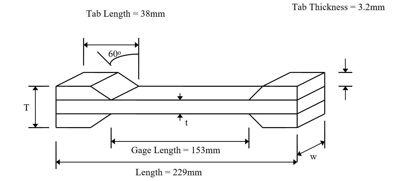
Figure 1 Schematic of Test Specimen used to find the Young’s modulus of a composite.
A tensile test geometry (Figure 1) to find the longitudinal tensile strength consists of 6-8 plies of \(0^{0}\) plies which are 12.5 mm (2 inches) wide and 229 mm (10 inches) long. The specimen is mounted with strain gages in the longitudinal and transverse direction. Tensile stresses are applied on the specimen at a rate of about 0.5 - 1 mm/min (0.02 to 0.04 in/min). A total of 40-50 data points for stress and strain are taken until a specimen fails. The stress in the longitudinal direction is plotted as a function of longitudinal strain as shown in Figure 2. The data is reduced using linear regression. The longitudinal Young’s modulus is the initial slope of the longitudinal stress, \(\sigma_{1}\) vs strain, longitudinal strain, \(\varepsilon_{1}\) curve.
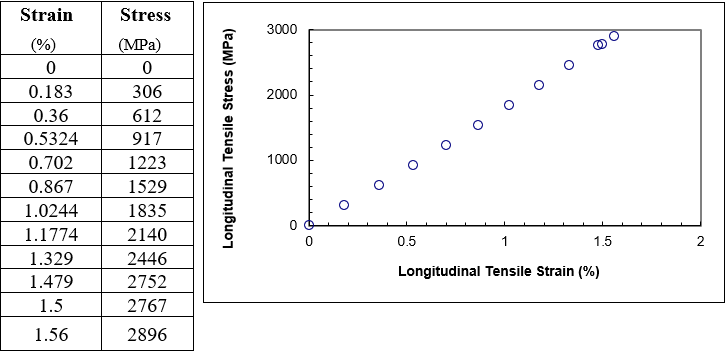
Figure 2 Longitudinal stress as a function of longitudinal strain for a graphite/epoxy composite.
The first order polynomial that one may fit to the data is
\[\sigma = E_{1}\varepsilon\ \ \ (1)\]
Questions
(1) Find the Young’s modulus, \(E_{1}\)?
(2) What is the longitudinal ultimate tensile strength?
(3) What is the longitudinal ultimate strain?
(4) What value of \(E_{1}\) do you get if you use the general linear regression model?
Modeling
Automated cartography deals with building or updating maps automatically from aerial or satellite images. Gone are the days when map updating was a laborious process that took a long period to accomplish. There are now many computer vision methods that one can employ to assist and ease the job of the cartographer. For instance, consider the aerial image shown, which is of a park with a lake. One of the tasks is to extract the road network that is visible. The road network appears as bright linear strips. On the right of that figure is shown the road network
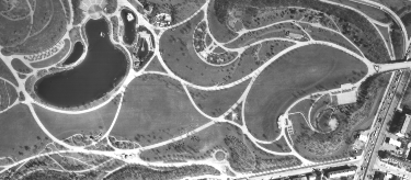

Figure 1. On left is an aerial image of park in Munich, Germany. We see the roads and a lake. On the right is the road network extracted from the image.
that is automatically extracted from the image. In this module, we will see how to achieve this by fitting models to the local intensities in the image.
Image is a collection of gray level values at set of predetermined sites known as pixels, arranged in an array. These gray level values are also known as image intensities. In the above figure we see the profile of the intensity value along a line (shown in red) cutting a road in an image. We represent small values to represent dark points in the image and large values to detect bright regions in the image. The value increases and then decreases. This intensity profile can be modeled as an inverted parabola. The road can be detected by identifying pixels in the image that exhibit this intensity profile around it. To detect all the road pixels, we would have to repeat this process for intensity profile along the vertical as well along the horizontal directions at each pixel.
Let the intensities profile at a pixel be denoted by the values:\(y_{- K},\ldots,y_{0},\ldots,y_{K}\), the index 0 is used to denote the pixel location under consideration and we look at K pixels on either sides of it. We will use \(x = - K,\ldots,0,\ldots K\) to denote these pixel locations that are the independent variables.
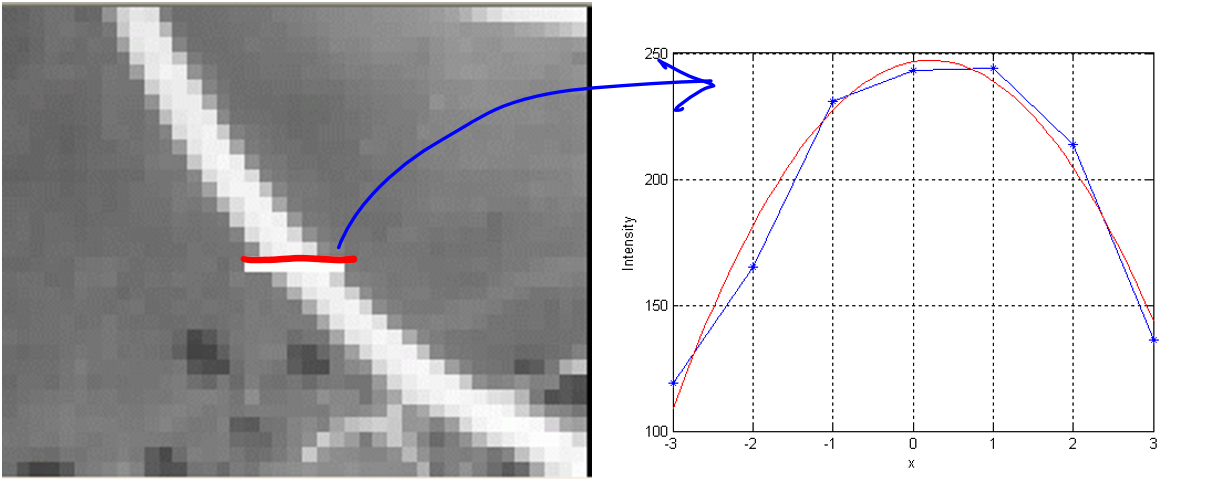
Figure 2. On left is a magnified portion of an image with a piece of the road. Note we can observe the individual pixels. On the right, we plot the intensities of the pixels marked by a red line. The raw intensities are plotted in blue, with fitted function in red.
Consider a polynomial model of the intensities.
\[y(x) = ax^{2} + bx + c\]
We fit this second order polynomial model to the observed intensities to minimize the fit error denoted by
\[\begin{split} e &= \sum_{k = - K}^{k = K}{(y_{k} - y(k))^{2}}\\ &=\sum_{k = - K}^{k = K}{(y_{k} - ak^{2} - {bk} - c)^{2}}\end{split}\]
The unknown parameters,\(a\), \(b\), and \(c\) can be estimated to be the values that minimize the above error. The necessary condition is that the derivative of the error with respect to these parameters be zero.
\[\frac{\partial e}{\partial a} = - \sum_{}^{}{2k^{2}(y_{k} - ak^{2} - {bk} - c)} = 0\]
\[\frac{\partial e}{\partial b} = - \sum_{}^{}{2k(y_{k} - ak^{2} - {bk} - c)} = 0\]
\[\frac{\partial e}{\partial c} = - \sum_{}^{}{2(y_{k} - ak^{2} - {bk} - c)} = 0\]
The three equations can be expressed in matrix form as
\[\begin{bmatrix} \displaystyle \sum_{k}^{}k^{4} & \displaystyle \sum_{k}^{}k^{3} & \displaystyle \sum_{k}^{}k^{2} \\ \displaystyle \sum_{k}^{}k^{3} & \displaystyle \sum_{k}^{}k^{2} & \displaystyle \sum_{k}^{}k^{1} \\ \displaystyle \sum_{k}^{}k^{2} & \displaystyle \sum_{k}^{}k^{1} & \displaystyle \sum_{k}^{}1 \\ \end{bmatrix}\begin{bmatrix} a \\ b \\ c \\ \end{bmatrix} = \begin{bmatrix} \displaystyle \sum_{k}^{}{k^{2}y_{k}} \\ \displaystyle \sum_{k}^{}{k^{\ }y_{k}} \\ \displaystyle \sum_{k}^{}y_{k} \\ \end{bmatrix}\]
We thus have three linear equations with three unknown, which can be solved using a variety of methods. The conditions corresponding to the road intensity profile, which is an inverted parabola, can be found by using the observation that the maximum of the fitted polynomial should happen at or near \(k = 0\). The condition for a maximum value is given by \(a < 0\) and the location of the maximum is given by \(- b/2a\), which should be between \(-0.5\) and \(0.5\) pixels. Note that \(0.5\) denotes the halfway location between the pixel at location \(0\) and the next pixel, which is at \(1\). The value of the maximum is given by \(c\), which should be high because we are looking of bright road edges.
Worked Out Example
Consider the following intensity profile: \({yk}= 119,\ 165,\ 231,\ 243,\ 244,\ 214,\ 136\) corresponding to \(k = - 3,\ - 2,\ - 1,\ 0,\ 1,\ 2,\ 3\). This intensity profile corresponds to the one shown in Figure 2. The corresponding simultaneous equation for best least square fit is given by
\[\begin{bmatrix} 196 & 0 & 28 \\ 0 & 28 & 0 \\ 28 & 0 & 0 \\ \end{bmatrix}\begin{bmatrix} a \\ b \\ c \\ \end{bmatrix} = \begin{bmatrix} 4286 \\ 162 \\ 1352 \\ \end{bmatrix}\]
The solution is given by \(a = - 13.3571,b = 5.7857,\) and \(c = 246.5714\). Since \(a\) is negative, we have a maximum value, which is located at \(- b/2a = - 0.2166\). This location is near \(0\) and the value at zero is \(246.57\), which denotes a bright value. All of these quantities suggest that we have a road at the pixel we are considering.
QUESTIONS
Instead of processing the an image, which is laid out in a 2D plane, along just the horizontal and vertical directions, it is more natural to consider fitting a 2D surface model, whose general form is given by
\[y(x,y) = ax^{2} + by^{2} + cxy + dx + ey + f\]
(1) Work out the regression equation for fitting this surface model to intensities in a \(K\) by \(K\) neighborhood around a pixel.
(2) How would you determine, based on the values of the estimated parameters, whether the pixel is on a road edge or not, that is, the fitted surface has a roof-like shape?
Summary
Many electrical devices have non-linear behavior. It is often advantageous to substitute a model for the device using simpler linear components. In the case of a diode, this is often done with a DC supply and a series resistor. To determine an appropriate value for the resistor, regression is used.
Modeling
All electrical devices exhibit non-linear behavior to some extent. This is caused by many factors including material and thermal properties. For most of the basic components, a simple linear model is used that is sufficient for most operating conditions. This is the case for resistors, capacitors, and inductors. Semiconductor devices, however, are specifically chosen for their non-linear behaviors. This allows them to perform gating, switching, and amplifying operations. Consider the case of a simple diode, like the 1N4001, whose forward-bias VI-characteristic is shown in Figure 1.
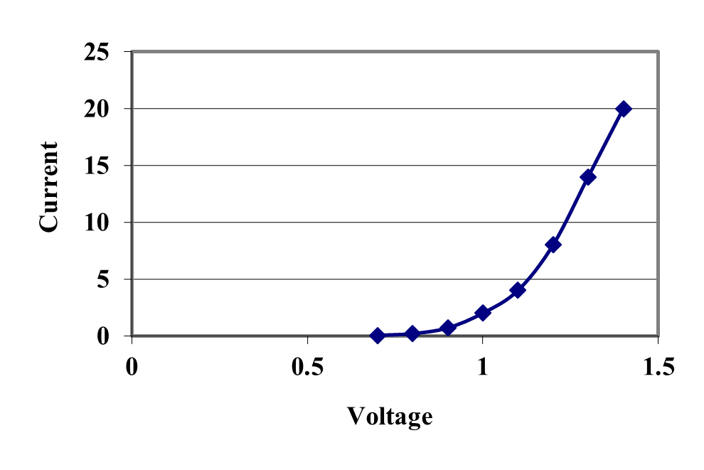
Figure 1 VI Forward-Bias Characteristic of a 1N4001 Diode [1]
In many applications it is suitable to model the forward-bias behavior of the diode as a simple voltage drop of about 0.7 V [2, pp. 70,1]. Other types of diodes, such as LEDs, have voltage drops on the order of 2.0 to 2.5 V. This modeling is not very realistic because it fails to account for the increasing voltage drop as current flow through the diode increases as is shown in Figure 1. If our analysis requires us to know how much current a diode can supply, then the ideal model is clearly inadequate.
It would be, of course, possible to model the diode using some form of interpolated curve, but that would almost certainly force any kind of analysis to be able to only use numerical tools. A much better solution would be to develop a model using simpler linear components that could be used in place of the diode. This is typically done using a DC supply and a series resistor as shown in Figure 2 [2, pp. 72-5].
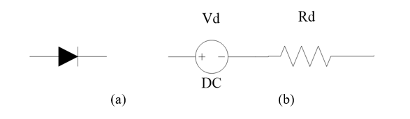
Figure 2. (a) Ideal Diode and (b) Forward Bias Model
The question then becomes, what are the appropriate values for \(V_{d}\) and \(R_{d}\)? The answer will vary from diode to diode, but good values can be determined using the numerical method of linear regression. The model of Figure 2b in effect replaces the characteristic of Figure 1 with that of Figure 3. Remember that for this to work we are still assuming the diode is sufficiently forward-biased to turn it on which means that the voltage across the diode must exceed \(V_{d}\).
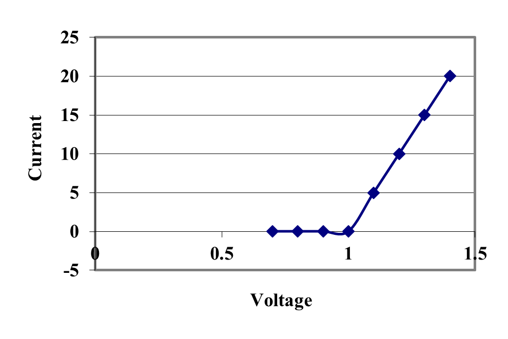
Figure 3. VI Characteristic of Forward Bias Model
Choosing suitable values for \(V_{d}\) and \(R_{d}\) will depend on the potential use for the diode. In a small signal application (low current) it would be more appropriate to choose current values from the original characteristic curve that are well-below 5 A. and for large-signal applications it would be a better fit to use current values of 5 A and above. To study this problem, let us take a closer look at the actual data used to generate the characteristic in Figure 1. This is shown in Table 1.
The simplest way to determine the \(V_{d}\) and \(R_{d}\) from the selected data is to generate a trend line for the region in question. This can be done using linear regression since a linear regression trend line has the effect of minimizing the mean-square error between the modeled line and the actual data. Using the standard linear regression model using \(\beta_{0}\) and \(\beta_{1}\) parameters yields the following equation for the trend line.
\[I \cong \beta_{1}V + \beta_{0}\]
Once \(\beta_{0}\) and \(\beta_{1}\)are known \(V_{d}\)and \(R_{d}\) can be computed as follows:
\[V_{d} = - \frac{\beta_{0}}{\beta_{1}}\]
\[R_{d} = \frac{1}{\beta_{1}}\]
Table 1. VI Characteristic of a Forward-Biased Diode
| Voltage, V | Current, A | Small Signal | Large Signal |
|---|---|---|---|
| \(0.0\) | \(0.00\) | \(N\) | \(N\) |
| \(0.6\) | \(0.01\) | \(Y\) | \(N\) |
| \(0.7\) | \(0.05\) | \(Y\) | \(N\) |
| \(0.8\) | \(0.20\) | \(Y\) | \(N\) |
| \(0.9\) | \(0.70\) | \(Y\) | \(Y\) |
| \(1.0\) | \(2.00\) | \(Y\) | \(Y\) |
| \(1.1\) | \(4.00\) | \(Y\) | \(Y\) |
| \(1.2\) | \(8.00\) | \(N\) | \(Y\) |
| \(1.3\) | \(14.00\) | \(N\) | \(Y\) |
| \(1.4\) | \(20.00\) | \(N\) | \(Y\) |
The effects of this choice are shown in Figure 4. When the data from the small-signal column of Table 1 is used to generate the regression line, it results in the model of Figure 4a and when the data from the large-signal column of Table 2 is used, the result is the model of Figure 4b.
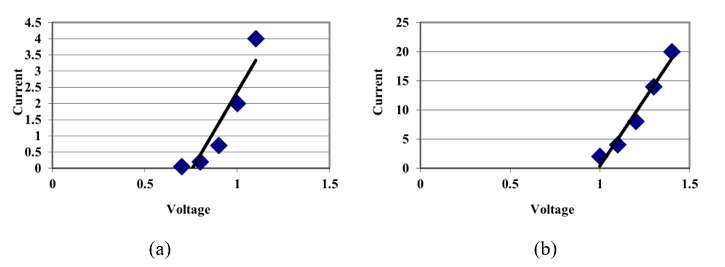
Figure 4 (a) Small-Signal Model and (b) Large-Signal Model for a Diode
The small-signal model agrees with the typical diode modeling where \(V_{d}\) is approximately 0.7V and will model the diode fairly well for currents below about 4 A. For a higher-current circuit the large-signal model with \(V_{d}\) approximately 1 V is a better choice, but will not model the data as well when the current is 2 A or below.
Complete the analysis by determining more exact values for \(V_{d}\) and \(R_{d}\) for both of these models. Use the small signal and large signal columns of Table 1 to select the data to use in your analysis.
Questions
(1) This analysis can be extended to handle other diodes. Find the data sheet for a 1N4150 or an LED, which shows the VI-Characteristic and derive suitable small- and large-signal forward-bias models.
(2) A similar analysis can be used to model the reverse-bias behavior of a diode. Use the datasheet from (1) to develop an appropriate model.
(3) Model the reverse-bias characteristics for a zener diode (e.g. the 1N4678 to 1N4717 family).
(4) The use of linear regression only reduces the modeling/approximating error for the sample data points provided. In this problem, we actually have a two-piece linear model (the flat portion up to \(V_{d}\) when the diode turns on and the forward-bias model involving \(R_{d}\) after the diode is on). This may not adequately model the entire forward-bias characteristic. Using your model values for \(V_{d}\) and \(R_{d}\) as a start, examine the overall characteristic and pick values for \(V_{d}\) and \(R_{d}\) that minimize the mean-square error over the entire forward bias region. This will have to be a combination of the error caused by having \(V_{d}\) to the right of the actual turn-on point as well as the error in the turned-on region. How close is this model to our simpler approach that modeled each piece separately?
References
[1] 1N4001 Data Sheet, Fairchild Semiconductor, http://www.fairchildsemi.com/ds/1N/1N4007.pdf, accessed May 12, 2005.
[2] Malvino, A., Electronic Principles, Sixth Edition, Glencoe McGraw-Hill, 1999.
Summary
Finding the number of toys a company should manufacture per day to maximize their injection molding and assembly line requires regression.
Modeling
An industrial engineer working for a manufacturing company has noticed a deviation in the accuracy of a machine after it runs for long periods without a cool down cycle. This is especially concerning because the company wants to increase production (longer machine operating times without a cool down) because of a large contract the company will start in 3-4 months. The industrial engineer decides to monitor the machining process to determine the point (hours of operation) when the machine is producing parts that could be out of tolerance. Over the course of several months, the industrial engineer monitored the machining process to determine a relationship between hours of machine use and millimeters off target the machine was. The data collected is shown in tabular form (Table 1) and scatter plot (Figure 1).
Table 1. Off target measured as a fubtion of machine use.
| Hours of Machine Use | Millimeters off Target |
|---|---|
| \(30\) | \(1.10\) |
| \(31\) | \(1.21\) |
| \(32\) | \(1.00\) |
| \(33\) | \(1.21\) |
| \(34\) | \(1.25\) |
| \(35\) | \(1.23\) |
| \(36\) | \(1.24\) |
| \(37\) | \(1.28\) |
| \(38\) | \(1.30\) |
| \(39\) | \(1.30\) |
| \(40\) | \(1.38\) |
| \(41\) | \(1.35\) |
| \(42\) | \(1.38\) |
| \(43\) | \(1.38\) |
| \(44\) | \(1.40\) |
| \(45\) | \(1.42\) |
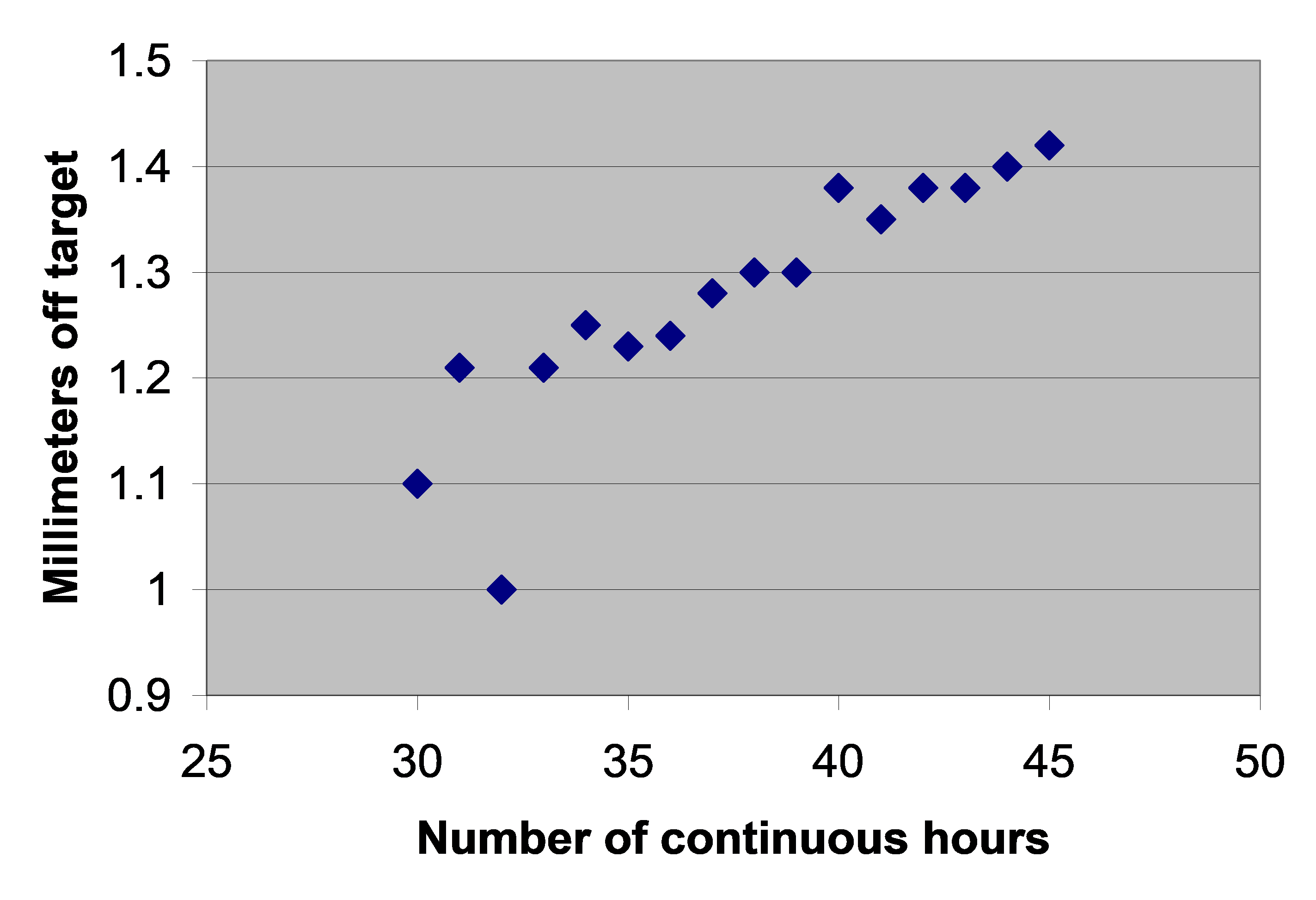
Figure 1. Off target measurement as a function of machine use.
Based on the above data, the industrial engineer would like to determine the number of hours of machine use that would produce a 2 millimeters off target because many parts would fail quality check at that point. Determine the number of hours of operation that produces 2 millimeter off target based on a least squares fit for the data.
Background
In order to determine a relationship between millimeters off target and hours of machine use, a curve (for example, a linear polynomial) needs to be fit to the data. This is done by regression where we best fit a curve through the data given in the previous table. In this case, we may best fit the data to a first order polynomial, that is
\[h = a_{0} + a_{1}t\]
Where \(h\) is the hours of machine use and \(t\) is the millimeters off target. The values of the coefficients in the above equations will be found by linear regression. Knowing the values of \(a_{0}\) and \(a_{1}\), we can determine the millimeters off target as a function of hours of machine use. For example, if we want to find the time when the machine will be 2 mm off target, then
\[2 = a_{0} + a_{1}t\]
giving
\[t = \frac{2 - a_{0}}{a_{1}}\]
Questions
(1) Fit the data in the previous table using a linear regression, and determine the hours of machine use that will make the machine 2 mm off target.
(2) Fit the data in the previous table using a second order polynomial regression, and determine the hours of machine use that will make the machine 2 millimeters off target.
(3) Find whether a linear or second order polynomial regression is a better fit to the data.
Summary
To find the diametrical contraction during shrink-fitting in a trunnion requires one to first find how the thermal expansion coefficient of steel is related to temperature. The relation is given through a second-order polynomial regression model.
Modeling
To make the fulcrum (Figure 1) of a bascule bridge, a long hollow steel shaft called the trunnion is shrink fit into a steel hub. The resulting steel trunnion-hub assembly is then shrink fit into the girder of the bridge.
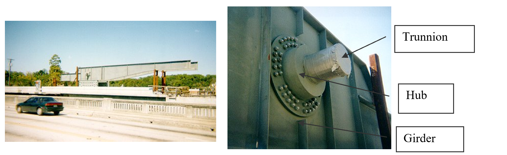
Figure 1 Trunnion-Hub-Girder (THG) assembly.
This shrink-fitting is done by first immersing the trunnion in a cold medium such as a dry-ice/alcohol mixture. After the trunnion reaches the steady-state temperature, that is, the temperature of the cold medium, the trunnion outer diameter contracts. The trunnion is taken out of the medium and slid through the hole of the hub (Figure 2).
When the trunnion heats up, it expands and creates an interference fit with the hub. In 1995, on one of the bridges in Florida, this assembly procedure did not work as designed. Before the trunnion could be inserted fully into the hub, the trunnion got stuck. Luckily, the trunnion was taken out before it got stuck permanently. Otherwise, a new trunnion and hub would be needed to be ordered at the cost of $50,000. Coupled with construction delays, the total loss could have been more than a hundred thousand dollars.
Why did the trunnion get stuck? This failure was because the trunnion had not contracted enough to slide through the hole. Can you find out why?
A hollow trunnion of outside diameter \({12.36}{3}{^{\prime\prime} }\) is to be fitted in a hub of inner diameter \(12.358{^{\prime\prime} }\). The trunnion was put in a dry ice/alcohol mixture (temperature of the fluid - dry ice/alcohol mixture is \(- 108{^\circ}\text{F}\)) to contract the trunnion so that it can be slid through the hole of the hub. To slide the trunnion without sticking, a diametrical clearance of at least \(0.01{^{\prime\prime} }\) is required between the trunnion and the hub. Assuming the room temperature is \(80{^\circ}\text{F}\), is immersing it in a dry-ice/alcohol mixture a correct decision?
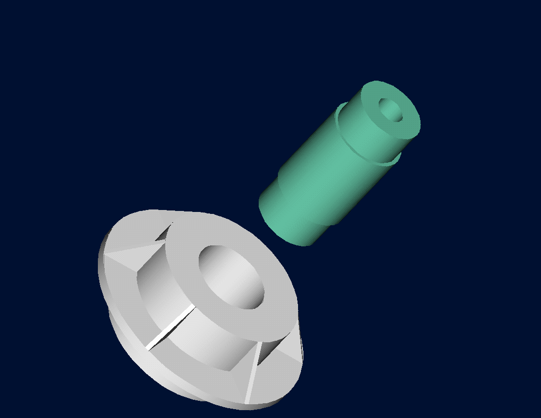
Figure 2 Trunnion slid through the hub after contracting.
Solution
To calculate the contraction in the diameter of the trunnion, coefficient of linear thermal expansion at room temperature is used. In that case the reduction, \({\Delta D}\) in the outer diameter of the trunnion is
\[\Delta D = D\alpha\Delta T\;\;\;\;\;\;\;\;\;\;\;\; (1)\]
where
\[D = \text{outer diameter of the trunnion,}\]
\[\alpha = \text{coefficient of linear thermal expansion at room temperature, and}\]
\[\Delta T = \text{change in temperature.}\]
Given
\[D = 12.363{^{\prime\prime} }\]
\[\alpha = 6.817 \times 10^{- 6}\ \text{in/in/}{^\circ}\text{F}\text{ at }80{^\circ}\text{F}\]
\[\begin{split} \Delta T&=T_{{fluid}} - T_{{room}}\\ &= - 188{^\circ}\text{F} \end{split}\]
where
\[T_{{fluid}} = \text{temperature of dry-ice/alcohol mixture,}\]
\[T_{{room}} = \text{room temperature,}\]
the reduction in the trunnion outer diameter (Equation 1) is given by
\[\begin{split} \Delta D &= (12.363)\left( 6.47 \times 10^{- 6} \right)\left( - 188 \right)\\ &= - 0.01504^{\prime\prime} \end{split}\]
So the trunnion is predicted to reduce in diameter by \(0.01504{^{\prime\prime} }\). But is this enough reduction in diameter? As per specifications, he needs the trunnion to contract by
\[\begin{split} &= \text{trunnion outside diameter - hub inner diameter + diametric clearance}\\ &= 12.363^{\prime\prime} - 12.358^{\prime\prime} + 0.01^{\prime\prime} \\ &= 0.015^{\prime\prime} \end{split}\]
So, according to his calculations, immersing the steel trunnion in a dry-ice/alcohol mixture gives the desired contraction of \(0.015^{\prime\prime}\) as we predict a contraction of \(0.01504{^{\prime\prime} }\).
But as shown in Figure 3 and Table 1, the coefficient of linear thermal expansion of steel decreases with temperature and is not constant over the range of temperature the trunnion goes through. Hence, the above formula (Equation 1) would overestimate the thermal contraction.
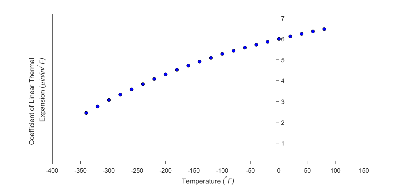
Figure 3 Varying coefficient of linear thermal expansion as a function of temperature for cast steel.
The contraction in the diameter for the trunnion for which the coefficient of linear thermal expansion varies as a function of temperature is given by
\[\Delta D = D\int_{T_{{room}}}^{T_{{fluid}}}{\alpha dT}\;\;\;\;\;\;\;\;\;\;\;\; (2)\]
So one needs to find the curve to find the coefficient of linear thermal expansion as a function of temperature. This curve is found by regression where we best fit a function through the data given in Table 1. In this case, we may fit a second-order polynomial
\[\alpha = a_{0} + a_{1} \times T + a_{2} \times T^{2}.\;\;\;\;\;\;\;\;\;\;\;\; (3)\]
The values of the coefficients in the above equations will be found by polynomial regression. Knowing the values of \(a_{0}\), \(a_{1}\),and \(a_{2}\), we can then find the contraction in the trunnion diameter from Equation (2) and (3) as
\[\begin{split} \Delta D &= D\int_{T_{{room}}}^{T_{{fluid}}}{(a_{0} + a_{1} \times T + a_{2} \times T^{2}})dT\\ &= D\lbrack a_{0} \times (T_{{fluid}} - T_{{room}}) + a_{1} \times \frac{({T_{{fluid}}}^{2} - {T_{{room}}}^{2})}{2} + a_{2} \times \frac{({T_{{fluid}}}^{3} - {T_{{room}}}^{3})}{3}\rbrack\;\;\;\;\;\;\;\;\;\;\;\; (4) \end{split}\]
Questions
(1) Find the contraction in the outer diameter of the trunnion.
(2) As required, is the magnitude of contraction more than \(0.015{^{\prime\prime} }\)?
(3) If the magnitude of the contraction is less than \(0.015{^{\prime\prime} }\), what if the trunnion were immersed in liquid nitrogen (boiling temperature\(= - 321{^\circ}F\))? Will that give enough contraction in the trunnion?
(4) Rather than regressing the data to a second-order polynomial so that one can find the contraction in the outer diameter of the trunnion, how would you use the trapezoidal rule of integration for unequal segments to find the contraction? What is the relative difference between the two results? The data for the coefficient of linear thermal expansion as a function of temperature is given in Table 1.
(5) We chose a second-order polynomial for regression. What would make a different order polynomial a better choice for regression? Is there an optimum order of polynomial you can find?
Table 1 Coefficient of linear thermal expansion as a function of temperature.
| Temperature | Coefficient of Thermal Expansion |
|---|---|
| \({^\circ}F\) | \({\mu}{in}{/}{in/}{{^\circ}}{F}\) |
| \(80\) | \(6.47\) |
| \(60\) | \(6.36\) |
| \(40\) | \(6.24\) |
| \(20\) | \(6.12\) |
| \(0\) | \(6.00\) |
| \(-20\) | \(5.86\) |
| \(-40\) | \(5.72\) |
| \(-60\) | \(5.58\) |
| \(-80\) | \(5.43\) |
| \(-100\) | \(5.28\) |
| \(-120\) | \(5.09\) |
| \(-140\) | \(4.91\) |
| \(-160\) | \(4.72\) |
| \(-180\) | \(4.52\) |
| \(-200\) | \(4.30\) |
| \(-220\) | \(4.08\) |
| \(-240\) | \(3.83\) |
| \(-260\) | \(3.58\) |
| \(-280\) | \(3.33\) |
| \(-300\) | \(3.07\) |
| \(-320\) | \(2.76\) |
| \(-340\) | \(2.45\) |