Chapter 08.02: Euler’s Method for Solving Ordinary Differential Equations
Learning Objectives
After successful completion of this lesson, you should be able to:
1) develop Euler’s method for solving first-order ordinary differential equations,
2) determine how the step size affects the accuracy of a solution, and
3) derive Euler’s method formula from the Taylor series
What is Euler’s method?
Euler’s method is a numerical technique to solve first-order ordinary differential equations of the form
\[\frac{dy}{dx} = f( x,y),y(x_0) = y_{0}\;\;\;\;\;\;\;\;\;\;\;\; (1)\]
Only first-order ordinary differential equations of the form given by Equation (1) can be solved by using Euler’s method. In another lesson, we discuss how Euler’s method is used to solve higher-order and coupled (simultaneous) ordinary differential equations.
How does one write a first-order differential equation in the above form?
Example 1
Rewrite
\[\frac{{dy}}{{dx}} + 2y = 1.3e^{- x},y\left( 0 \right) = 5\]
in
\[\frac{{dy}}{{dx}} = f(x,y),\ y(0) = y_{0}\ \text{form.}\]
Solution
\[\frac{{dy}}{{dx}} + 2y = 1.3e^{- x},y\left( 0 \right) = 5\]
\[\frac{{dy}}{{dx}} = 1.3e^{- x} - 2y,y\left( 0 \right) = 5\]
In this case
\[f\left( x,y \right) = 1.3e^{- x} - 2y\]
Example 2
Rewrite
\[e^{y}\frac{{dy}}{{dx}} + x^{2}y^{2} = 2\sin(3x),\ y\left( 0 \right) = 5\]
in
\[\frac{{dy}}{{dx}} = f(x,y),\ y(0) = y_{0}\ \text{form.}\]
Solution
\[e^{y}\frac{{dy}}{{dx}} + x^{2}y^{2} = 2\sin(3x),\ y\left( 0 \right) = 5\]
\[\frac{{dy}}{{dx}} = \frac{2\sin(3x) - x^{2}y^{2}}{e^{y}},\ y\left( 0 \right) = 5\]
In this case
\[f\left( x,y \right) = \frac{2\sin(3x) - x^{2}y^{2}}{e^{y}}\]
Derivation of Euler’s method
At \(x = 0\), we are given the value of \(y = y_{0}.\) Let us call \(x = 0\) as \(x_{0}\). Now since we know the slope of \(y\) with respect to \(x\), that is, \(f\left( x,y \right)\), then at \(x = x_{0}\), the slope is \(f\left( x_{0},y_{0} \right)\). Both \(x_{0}\) and \(y_{0}\) are known from the initial condition \(y\left( x_{0} \right) = y_{0}\).
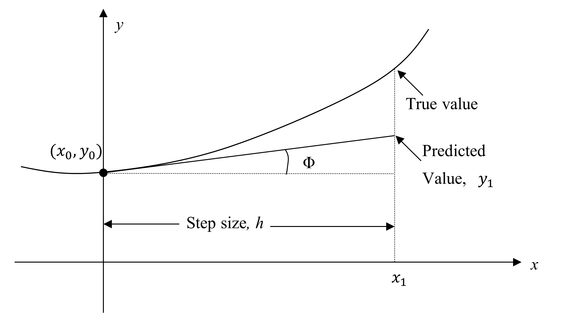
Figure 1 Graphical interpretation of the first step of Euler’s method.
So the slope at \(x = x_{0},\) as shown in Figure 1, is
\[\begin{split} Slope,\left.\frac{dy}{dx}\right|_{x_0,y_0} &= \frac{\text{Rise}}{\text{Run}}\\ &= \frac{y_{1} - y_{0}}{x_{1} - x_{0}}\\ &= f\left( x_{0},y_{0} \right) \end{split}\]
So
\[\frac{y_{1} - y_{0}}{x_{1} - x_{0}}= f\left( x_{0},y_{0} \right)\]
gives
\[y_{1} = y_{0} + f\left( x_{0},y_{0} \right)\left( x_{1} - x_{0} \right)\]
Calling \(x_{1} - x_{0}\) the step size \(h\), we get
\[y_{1} = y_{0} + f\left( x_{0},y_{0} \right)h\;\;\;\;\;\;\;\;\;\;\;\; (2)\]
One can now use the value of \(y_{1}\) (an approximate value of \(y\) at \(x = x_{1}\)) to calculate \(y_{2}\), and that would be the predicted value at \(x_{2}\), given by
\[y_{2} = y_{1} + f\left( x_{1},y_{1} \right)h\]
\[x_{2} = x_{1} + h\]
Based on the above equations, if we now know the estimated value of \(y\) at \(x_{i}\) as \(y_i\), then
\[y_{i + 1} = y_{i} + f\left( x_{i},y_{i} \right)h\;\;\;\;\;\;\;\;\;\;\;\; (3)\]
Equation (3) is known as Euler’s method and is illustrated graphically in Figure 2. In some textbooks, it is also called the Euler-Cauchy method.
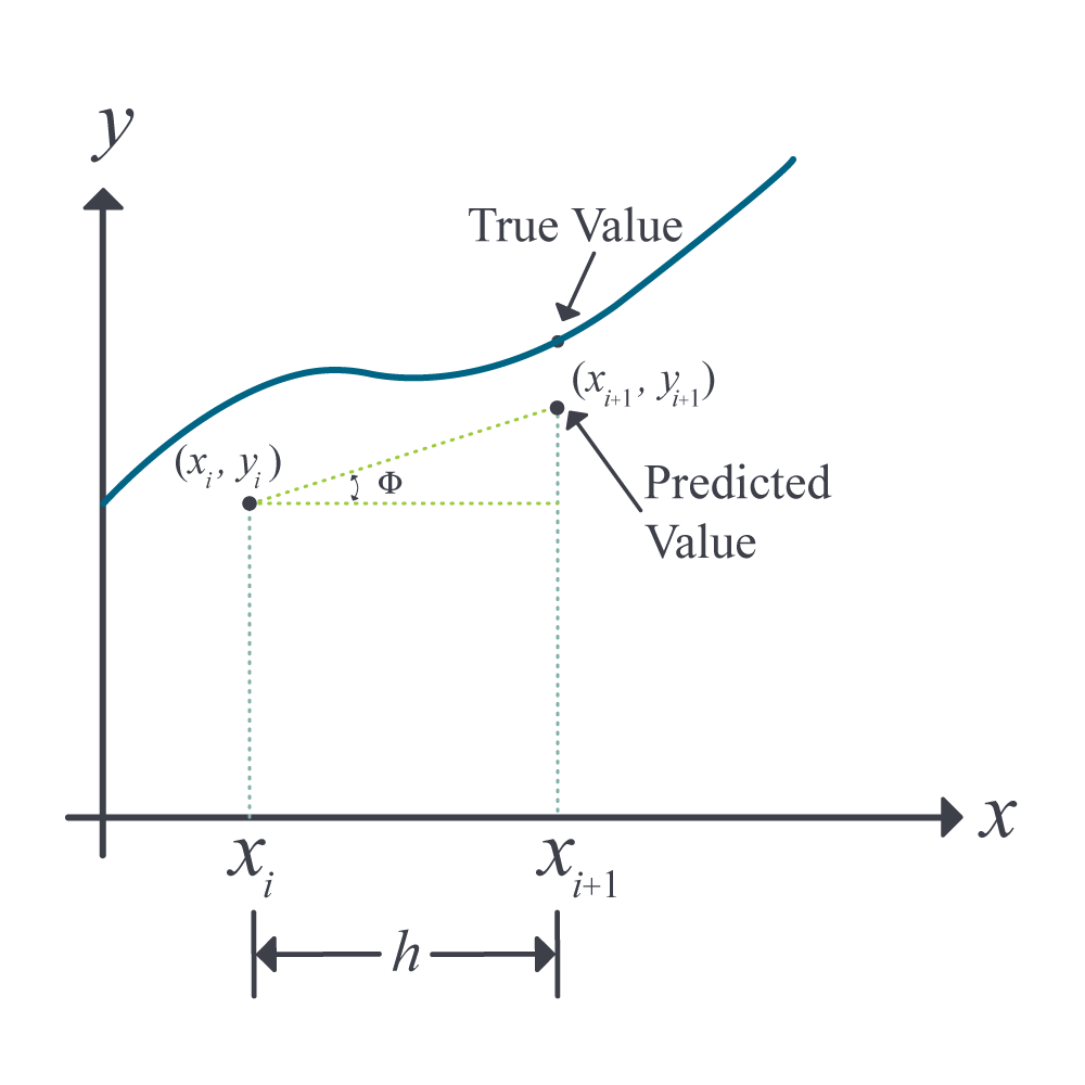
Figure 2 General graphical interpretation of Euler’s method.
Derivation of Euler’s Method from Taylor Series
Euler’s method can be derived from the Taylor series as follows.
\[y_{i + 1} = y_{i} + \left. \ \frac{{dy}}{{dx}} \right|_{x_{i},y_{i}}\left( x_{i + 1} - x_{i} \right) + \frac{1}{2!}\left. \ \frac{d^{2}y}{dx^{2}} \right|_{x_{i},y_{i}}\left( x_{i + 1} - x_{i} \right)^{2} + \frac{1}{3!}\left. \ \frac{d^{3}y}{dx^{3}} \right|_{x_{i},y_{i}}\left( x_{i + 1} - x_{i} \right)^{3} + ...\;\;\;\;\;\;\;\;\;\;\;\; (5)\]
Since \(\displaystyle \frac{dy}{dx} = f{(x,y)}\)
\[y_{i+1}= y_{i} + f(x_{i},y_{i})(x_{i + 1} - x_{i}) + \frac{1}{2!}f^\prime(x_{i},y_{i})\left( x_{i + 1} - x_{i} \right)^{2} + \frac{1}{3!}f^{\prime\prime}(x_{i},y_{i})\left( x_{i + 1} - x_{i} \right)^{3} + ...\;\;\;\;\;\;\;\;\;\;\;\; (6)\]
As you can see, using only the first two terms of the Taylor series in Equation (6)
\[y_{i + 1} = y_{i} + f\left( x_{i},y_{i} \right)h\;\;\;\;\;\;\;\;\;\;\;\; (3-repeated)\]
is the Euler’s method.
The true error in the Euler’s method hence is given by
\[E_{t} = \frac{f^{\prime}\left( x_{i},y_{i} \right)}{2!}h^{2} + \frac{f^{\prime\prime}\left( x_{i},y_{i} \right)}{3!}h^{3} + ...\;\;\;\;\;\;\;\;\;\;\;\; (7)\]
The true error hence is approximately proportional to the square of the step size. That is, as the step size is halved, the true error gets approximately quartered. However, we will observe that as the step size gets halved, the true error instead only gets approximately halved. This reduction in accuracy is because the true error, being proportional to the square of the step size, is the local truncation error, that is, the error from one point to the next. The global truncation error is, however, proportional only to the step size as the error keeps propagating through the \(n\) steps taken from the initial value of \(x=x_0\) to the final value \(x=x_n\).
Learning Objectives
After successful completion of this lesson, you should be able to:
1) Use Euler’s Method to solve a first-order ordinary differential equation.
Recap of Euler’s Method
In the previous lesson, we discussed the theory behind Euler’s method of solving an ordinary differential equation of the from \(\displaystyle \frac{dy}{dx}=f(x,y)\) where \(y(x_0)=y_0\). In this lesson, we illustrate how to apply the algorithm of Euler’s method.
Example 1
A ball at \(1200\ \text{K}\) is allowed to cool down in air at an ambient temperature of \(300\ \text{K}\). Assuming heat is lost only due to radiation, the differential equation for the temperature of the ball is given by
\[\frac{{d\theta }}{{dt}} = - 2.2067 \times 10^{- 12}\left( \theta^{4} - 81 \times 10^{8} \right),\ \theta\left( 0 \right) = 1200\ \text{K} \;\;\;\;\;\;\;\;\;\;\;\; (E1.1)\]
where \(\theta\) is in \(K\) and \(t\) in seconds. Find the temperature at \(t = 480\) seconds using Euler’s method. Assume a step size of \(h = 240\) seconds. Compare with the exact value.
Solution
\[\frac{{d\theta }}{{dt}} = - 2.2067 \times 10^{- 12}\left( \theta^{4} - 81 \times 10^{8} \right)\]
\[f\left( t,\theta \right) = - 2.2067 \times 10^{- 12}\left( \theta^{4} - 81 \times 10^{8} \right)\]
Euler’s method formula is
\[\theta_{i + 1} = \theta_{i} + f\left( t_{i},\theta_{i} \right)h\]
For \(i = 0\), \(t_{0} = 0\), \(\theta_{0} = 1200\)
\[\begin{split} \theta_{1} &= \theta_{0} + f\left( t_{0},\theta_{0} \right)h\\ &= 1200 + f\left( 0,1200 \right) \times 240\\ &= 1200 + \left( - 2.2067 \times 10^{- 12}\left( 1200^{4} - 81 \times 10^{8} \right) \right) \times 240\\ &= 1200 + \left( - 4.5579 \right) \times 240\\ &= 106.09\ \ \text{K} \end{split}\]
\(\theta_{1}\) is the approximate temperature at
\[t = t_{1} = t_{0} + h = 0 + 240 = 240\ \text{s}\]
\[\theta_{1} = \theta\left( 240 \right) \approx 106.09\ \text{K}\]
For \(i = 1\), \(t_{1} = 240\), \(\theta_{1} = 106.09\)
\[\begin{split} \theta_{2} &= \theta_{1} + f\left( t_{1},\theta_{1} \right)h\\ &= 106.09 + f\left( 240,106.09 \right) \times 240\\ &= 106.09 + \left( - 2.2067 \times 10^{- 12}\left( 106.09^{4} - 81 \times 10^{8} \right) \right) \times 240\\ &= 106.09 + \left( 0.017595 \right) \times 240\\ &= 110.32\ \ \text{K} \end{split}\]
\(\theta_{2}\) is the approximate temperature at
\[t = t_{2} = t_{1} + h = 240 + 240 = 480\ \text{s}\]
\[\theta_{2} = \theta\left( 480 \right) \approx 110.32\ \text{K}\]
The exact solution of the ordinary differential Equation (E1.1) is given without proof as the solution of the nonlinear equation
\[0.92593\ln\frac{\theta - 300}{\theta + 300} - 1.8519\tan^{- 1}\left( 0.333 \times 10^{- 2}\theta \right) = - 0.22067 \times 10^{- 3}t - 2.9282\;\;\;\;\;\;\;\;\;\;\;\; (E1.2)\]
The solution to the nonlinear Equation (E1.2) at \(t=480 \ \text{s}\) is
\[\theta_{exact} = 647.57\ \text{K}\] Figure 1 compares the exact solution (\(647.57\ \text{K}\)) with the numerical solution from Euler’s method for the step size of \(h = 240\).
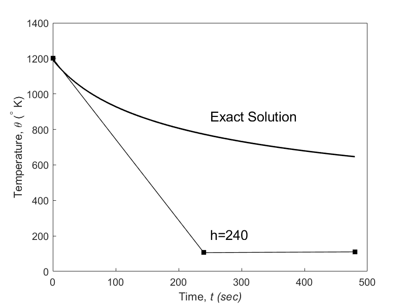
Figure 1 Comparing the exact and Euler’s method solutions.
The problem was solved again using a smaller step size. The results are given below in Table 1.
Table 1 Temperature at \(480\) seconds as a function of step size, \(h\).
| \(\text{Step size},\) \(h\) | \(\theta\left( 480 \right)\) | \(E_{t}\) | \(| \epsilon_{t}|\%\) |
|---|---|---|---|
\(480\) \(240\) \(120\) \(60\) \(30\) |
\(-987.81\) \(110.32\) \(546.77\) \(614.97\) \(632.77\) |
\(1635.4\) \(537.26\) \(100.80\) \(32.607\) \(14.806\) |
\(252.54\) \(82.964\) \(15.566\) \(5.0352\) \(2.2864\) |
Figure 2 shows how the temperature varies as a function of time for different step sizes.
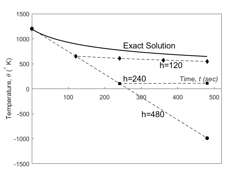
Figure 2 Comparison of Euler’s method with the exact solution for different step sizes.
The values of the calculated temperature at \(t = 480\ \text{s}\) as a function of step size are plotted in Figure 3.
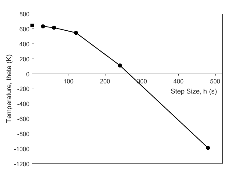
Figure 3 Effect of step size in Euler’s method.
It can be seen that Euler’s method results have large errors. In the previous lesson, we found that the true error in the approximation is given by
\[E_{t} = \frac{f^{\prime}\left( x_{i},y_{i} \right)}{2!}h^{2} + \frac{f^{\prime\prime}\left( x_{i},y_{i} \right)}{3!}h^{3} + ...\;\;\;\;\;\;\;\;\;\;\;\; (2)\]
The true error hence is approximately proportional to the square of the step size. That is, as the step size is halved, the true error gets approximately quartered. However, from Table 1, we see that as the step size gets halved, the true error only gets approximately halved (closer to when the step size becomes reasonable). This reduction in accuracy is because the true error, being proportional to the square of the step size, is the local truncation error, that is, the error from one point to the next. The global truncation error is, however, proportional only to the step size as the error keeps propagating through the \(n\) steps taken from the initial condition value of \(x=x_0\) to \(x=x_n\).
Learning Objectives
After successful completion of this lesson, you should be able to:
1) use Euler’s method to find the approximate value of a definite integral.
Introduction
In an earlier lesson, when asked to find \(\displaystyle \int_{a}^{b}{f\left( x \right){dx}}\), we could rewrite the integral as the solution of an ordinary differential equation (here is where we are using the first part of the fundamental theorem of calculus)
\[\frac{{dy}}{{dx}} = f\left( x \right),{\ }y(a) = 0,\;\;\;\;\;\;\;\;\;\;\;\; (1)\]
where then \(y\left( b \right)\) (here is where we are using the second part of the fundamental theorem of calculus) gives us the value of the integral \(\displaystyle \int_{a}^{b}{f\left( x \right){dx}}\).
Example 1
Find an approximate value of
\[\displaystyle \int_{5}^{8}{6x^{3}{dx}}\]
using Euler’s method of solving an ordinary differential equation. Use a step size of \(h = 1.5\).
Solution
Given \(\displaystyle \int_{5}^{8}{6x^{3}{dx}}\), we can rewrite the integral as the solution of an ordinary differential equation
\[\frac{{dy}}{{dx}} = 6x^{3},y\left( 5 \right) = 0\]
where \(y\left( 8 \right)\) gives the value of the integral \(\displaystyle \int_{5}^{8}{6x^{3}{dx}}\).
\[\frac{{dy}}{{dx}} = 6x^{3} = f\left( x,y \right),\ y\left( 5 \right) = 0\]
The Euler’s method formula is
\[y_{i + 1} = y_{i} + f\left( x_{i},y_{i} \right)h\]
Step 1
\[i = 0,\ x_{0} = 5,y_{0} = 0\] \[h = 1.5 \]
\[\begin{split} x_{1} &= x_{0} + h\\ &= 5 + 1.5\\ &= 6.5 \end{split}\]
\[y_{1} = y_{0} + f\left( x_{0},y_{0} \right)h\] \[\begin{split} y_{1} &= 0 + f\left( 5,0 \right)\times1.5\\ &= 0 + f\left( 6\times5^{3} \right)\times1.5\\ &=1125\\ &\approx y(6.5) \end{split}\] Step 2
\[i = 1,x_{1} = 6.5,y_{1} = 1125\]
\[\begin{split} x_{2} &= x_{1} + h\\ &= 6.5 + 1.5\\ &= 8 \end{split}\]
\[\begin{split} y_{2} &= y_{1} + f\left( x_{1},y_{1} \right)h\\ &= 1125 + f\left( 6.5,1125 \right)\times1.5\\ &= 1125 + f\left( 6\times6.5^3 \right)\times1.5\\ &=3596.625\\ &\approx y(8)\end{split}\]
Hence
\[\begin{split} \int_{5}^{8}{6x^{3}}dx &= y(8) - y(5)\\ &\approx 3596.625 - 0\\ &=3596.625\end{split}\]
Multiple Choice Test
(1). To solve the ordinary differential equation
\[3\frac{{dy}}{{dx}} + 5y^{2} = \sin x,\ y\left( 0 \right) = 5\]
by Euler’s method, you need to rewrite the equation as
(A) \(\displaystyle \frac{{dy}}{{dx}} = \sin x - 5y^{2},\ y\left( 0 \right) = 5\)
(B) \(\displaystyle \frac{{dy}}{{dx}} = \frac{1}{3}\left( \sin x - 5y^{2} \right),\ y\left( 0 \right) = 5\)
(C) \(\displaystyle \frac{{dy}}{{dx}} = \frac{1}{3}\left( - \cos x - \frac{5y^{3}}{3} \right),\ y\left( 0 \right) = 5\)
(D) \(\displaystyle \frac{{dy}}{{dx}} = \frac{1}{3}\sin x,\ y\left( 0 \right) = 5\)
(2). Given
\[3\frac{{dy}}{{dx}} + 5y^{2} = \sin x,\ y\left( 0.3 \right) = 5\]
and using a step size of \(h = 0.3\), the value of \(y\left( 0.9 \right)\) using Euler’s method is most nearly
(A) \(-35.318\)
(B) \(-36.458\)
(C) \(-658.91\)
(D) \(-669.05\)
(3). Given
\[3\frac{{dy}}{{dx}} + \sqrt{y} = e^{0.1x},\ y\left( 0.3 \right) = 5\]
and using a step size of \(h = 0.3\), the best estimate of \(\displaystyle \frac{{dy}}{{dx}}\left( 0.9 \right)\) using Euler’s method is most nearly
(A) \(- 0.37319\)
(B) \(- 0.36288\)
(C) \(- 0.35381\)
(D) \(- 0.34341\)
(4). The velocity \((m/s)\) of a body is given as a function of time (seconds) by
\[v\left( t \right) = 200\ln\left( 1 + t \right) - t,\ t \geq 0\]
Using Euler’s method with a step size of 5 seconds, the distance traveled in meters by the body from \(t = 2\ \text{s}\) to \(t = 12 \text{ s}\) is most nearly
(A) \(3133.1\)
(B) \(3939.7\)
(C) \(5638.0\)
(D) \(39397\)
(5). Euler’s method can be derived by using the first two terms of the Taylor series of writing the value of \(y_{i + 1}\), that is, the value of \(y\) at \(x_{i + 1}\), in terms of \(y_{i}\) and all the derivatives of \(y\) at \(x_{i}\). If \(h = x_{i + 1} - x_{i}\), the explicit expression for \(y_{i + 1}\) if the first three terms of the Taylor series are chosen to solve the ordinary differential equation
\[2\frac{{dy}}{{dx}} + 3y = e^{- 5x},\ y\left( 0 \right) = 7\]
would be
(A) \(\displaystyle y_{i + 1} = y_{i} + \frac{1}{2}\left( e^{- 5x_{i}} - 3y_{i} \right)h\)
(B) \(\displaystyle y_{i + 1} = y_{i} + \frac{1}{2}\left( e^{- 5x_{i}} - 3y_{i} \right)h - \frac{1}{2}\left( \frac{5}{2}e^{- 5x_{i}} \right)h^{2}\)
(C) \(\displaystyle y_{i + 1} = y_{i} + \frac{1}{2}\left( e^{- 5x_{i}} - 3y_{i} \right)h + \frac{1}{2}\left( - \frac{13}{4}e^{- 5x_{i}} + \frac{9}{4}y_{i} \right)h^{2}\)
(D) \(\displaystyle y_{i + 1} = y_{i} + \frac{1}{2}\left( e^{- 5x_{i}} - 3y_{i} \right)h - \frac{3}{2}y_{i}h^{2}\)
(6). A homicide victim is found at \(6:00\ \text{PM}\) in an office building that is maintained at \(72^{\circ} \text{F}\). When the victim was found, his body temperature was measured to be \(85^{\circ} \text{F}\). Three hours later, at \(9:00\ \text{PM}\), his body temperature was recorded at \(78^{\circ} \text{F}\). Assume the temperature of the body at the time of death is the normal human body temperature of \(98.6^{\circ} \text{F}\).
The governing equation for the temperature \(\theta\) of the body is
\[\displaystyle \frac{{d\theta }}{{dt}} = - k(\theta - \theta_{a})\]
where
\[\theta = \text{temperature of the body,}\ ^\circ \text{F}\]
\[\theta_a = \text{ambient temperature,}\ ^{\circ} \text{F}\]
\[t = \text{time,}\ \text{hrs}\]
\[k = \text{constant based on thermal properties of the body and air}, \text{1/s}\]
The estimated time of death most nearly is
(A) \(2:11\ \text{PM}\)
(B) \(3:13\ \text{PM}\)
(C) \(4:34\ \text{PM}\)
(D) \(5:12\ \text{PM}\)
For the complete solution, go to
http://nm.mathforcollege.com/mcquizzes/08ode/quiz_08ode_euler_solution.pdf
Problem Set
(1). For the ordinary differential equation
\[2\frac{dy}{dx} + 3xy = e^{- 1.5x},y(0) = 5,\]
use a step size of \(h = 2\) and the Euler’s method to find \(y(6)\).
Answer: \(329.45\)
2). For the ordinary differential equation
\[2\frac{dy}{dx} + 3 y = e^{- 1.5x},y(0) = 5\]
a) use Euler’s method to find \(y(2.5)\) using \(h = 1.25\),
b) use Euler’s method to find \(\displaystyle \frac{dy}{dx}\ (2.5)\) using \(h = 1.25\),
c) true value of \(y(2.5)\),
d) absolute relative true error for part (a),
e) true value of \(\displaystyle \frac{dy}{dx} (2.5)\),
f) absolute relative true error for part (b).
Answer: \(a)\ 3.371\)
\(b)\ -5.0539\)
\(c)\ 0.14699\)
\(d)\ 2197.6\%\)
\(e)\ -0.20872\)
\(f)\ 2321.4\%\)
(3). Find the approximate value of the integral \(\int_{3}^{8}{2e^{0.6x}dx}\) using Euler’s method.
a) Use \(h = 2.5\) and compare the value with the exact value.
b) Use \(h = 1.25\) and compare the value with the exact value.
Answer: \(a)\ 165.81\), true value=\(384.87\), true error=\(219.06\)
\(b)\ 258.42\), true value=\(384.87\), true error=\(126.45\)
(4). From problem (3a), is the value obtained using Euler’s method the same as 2-segment LRAM (Left Endpoint Rectangular Approximation), or 2-segment MRAM (Midpoint Rectangular Approximation), or 2-segment RRAM (Right Endpoint Rectangular Approximation) method of integration or the composite trapezoidal rule with 2-segments? Explain.
Answer: \(165.81\), same as LRAM
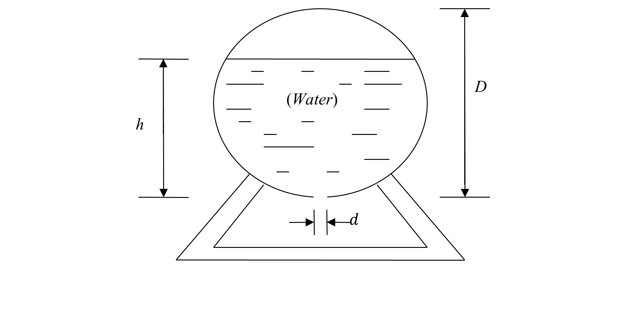
(5). A water tank with a hole at the top and a circular hole at the bottom is shown in the figure.
Given
\[\text{Diameter of the tank,}\ D = 6\ \text{m}\]
\[\text{Initial height of the water,}\ h = 5\ \text{m}\]
\[\text{Diameter of the hole,}\ d = 4.95\ \text{cm}\]
The flow rate \(\dot{Q}\) of water through the bottom hole is given by
\[\dot{Q} = - Av,\]
where
\[A =\text{cross-sectional area of the hole,}\]
\[v =\text{velocity of the water flowing through the hole.}\]
Since
\[v = \sqrt{2gh}\]
where
\[h =\text{height of water from the bottom of the tank,}\]
\[g =\text{acceleration due to gravity.}\]
From this, we get
\[\dot{Q} = - A\sqrt{2gh}\]
Also, since the volume \(V\) of the water at height \(h\) is given by
\[V = \frac{1}{3}\pi h^{2}\left( \frac{3D}{2} - h \right)\]
where
\[\frac{dV}{dt} = \left( \pi hD - \pi h^{2} \right)\frac{dh}{dt}\]
Since
\[\dot{Q} = \frac{dV}{dt}\]
\[\left( \pi hD - \pi h^{2} \right)\frac{dh}{dt} = - A\sqrt{2gh}\]
\[\left( \pi hD - \pi h^{2} \right)\frac{dh}{dt} = - \frac{\pi d^{2}}{4}\sqrt{2gh}\]
\[\frac{dh}{{dt}} = - \frac{d^{2}\sqrt{2gh}}{4\left( hD - h^{2} \right)}\]
a) Use Euler’s method with a step size of \(10\) minutes to find the height of water at \(t = 50\) minutes.
b) Based on the result from part (a), estimate the time at which the height of the water is 4 m.
c) Compare the results of part (a) and part (b) with the exact values.
Answer: \(a)\ 2.7737\ \ \text{m}\)
\(b)\ 15.965\ \text{minutes}\)
\(c)\) part (a) exact \(2.9371 \ \text{m}\), \(|\epsilon_t|=5.5623\%\)
part (b) exact \(19.415\ \text{minutes}\), \(|\epsilon_t|=21.802\%\)
(6). A spherical ball is taken out of a furnace at \(2500\ \text{K}\). It loses heat due to radiation and convection. Given the following,
\[\text{Radius of ball,}\ r = 1.0\ \text{cm}\]
\[\text{Density of the ball,}\ \rho = 3000\ \text{kg/m}^{3}\]
\[\text{Specific heat,}\ C = 1000\ \text{J}/(\text{kg} \cdot \text{K})\]
\[\text{Emittance,}\ \in = 0.5\]
\[\text{Stefan-Boltzmann Constant,}\ \sigma = 5.67 \times 10^{- 8}\ \text{J}/(\text{s} \cdot \text{m}^{2} \cdot \text{K}^{4})\]
\[\text{Convective cooling coefficient,}\ h = 500\ \text{J}/(\text{s} \cdot \text{m}^{2} \cdot \text{K})\]
\[\text{Initial temperature of the ball,}\ \theta(0) = 2500\ \text{K},\]
\[\text{Ambient temperature,}\ \theta_{a} = 300\ \text{K},\]
the ordinary differential equation that governs the temperature of the ball is given by
\[\frac{d\theta}{dt} = - 2.8349 \times 10^{- 12}(\theta^{4} - 81 \times 10^{8}) - 0.05(\theta - 300).\]
Hint: The above formula was calculated by using the knowledge that
\[\text{Rate of heat lost due to radiation}\ = A \in \sigma(\theta^{4} - \theta_{a}^{4})\]
\[\text{Rate of heat lost due to convection}\ = hA(\theta - \theta_{a})\]
\[\text{Heat stored}\ = mc\theta\]
where
\[A =\text{surface area of the ball,}\]
\[m =\text{mass of the ball.}\]
a) What are following at \(t = 0\ \text{s}\)?
temperature,
rate of change of temperature,
rate of heat loss due to radiation,
rate of heat loss due to convection,
rate of heat stored.
b) Find the following at \(t = 10\ \text{s}\) using Euler’s method and a step size of \(h = 2.5\).
temperature,
rate of change of temperature,
rate of heat loss due to radiation,
rate of heat loss due to convection,
rate of heat stored.
c) Can either convection or radiation be neglected if we are interested in finding the temperature profile between \(0\) and \(10\ \text{s}\)? Base your answer on quantitative reasoning.
d) Find the time when the temperature will be \(2000\ \text{K}\) using Euler’s method with a step size of \(h = 2.5\).
Answer:
\(a)\ 2500\ \text{K},\ -220.72\ \text{K/s},\ 1391.3\ \text{W},\ 1382.3\ \text{W},\ -2773.6\ \text{W}\)
\(b)\ 1252.3\ \text{K},\ -54.568\ \text{K/s},\ 87.344\ \text{W},\ 598.38\ \text{W},\ -685.72\ \text{W}\)
\(c)\) Neither can be ignored, as the rate of heat lost due to convection and radiation are of the
same order.
\(d)\ 2.2654\ \text{s}\) using linear interpolation