Chapter 08.01: Prerequisites to Numerical Methods for Solving Ordinary Differential Equations
Learning Objectives
After successful completion of this lesson, you should be able to:
1) find why some mathematical models are given by ordinary differential equations
Introduction
Differential equations have applications in all areas of science and engineering. A mathematical formulation of most of the physical and engineering problems leads to differential equations. So, it is crucial for engineers and scientists to know how to set up differential equations and solve them.
An equation that consists of derivatives is called a differential equation, and they are of two types
- ordinary differential equations (ODE)
- partial differential equations (PDE)
An ordinary differential equation has only one independent variable. Examples of ordinary differential equations include
\[\frac{d^{2}y}{dx^{2}} + 2\frac{{dy}}{{dx}} + y = 0, \frac{{dy}}{{dx}}(0) = 2,\ y(0) = 4,\]
\[\frac{d^{3}y}{dx^{3}} + 3\frac{d^{2}y}{dx^{2}} + 5\frac{{dy}}{{dx}} + y = \sin x,\ \frac{d^{2}y}{dx^{2}}(0) = 12,\ \frac{{dy}}{{dx}}(0) = 2,\ y(0) = 4\]
where \(x\) is the independent variable, and \(y\) is the dependent variable.
Ordinary differential equations are classified in terms of order and degree. The order of an ordinary differential equation is the same as the highest derivative, and the degree of an ordinary differential equation is the power of the highest derivative. Thus the differential equation,
\[x^{3}\frac{d^{3}y}{dx^{3}} + x^{2}\frac{d^{2}y}{dx^{2}} + x\frac{{dy}}{{dx}} + xy = e^{x}\]
is of order 3 and degree 1, whereas the differential equation
\[\left( \frac{{dy}}{{dx}} + 1 \right)^{2} + x^{2}\frac{{dy}}{{dx}} = \sin x\]
is of order 1 and degree 2.
An engineer’s approach to differential equations is different from a mathematician. While the latter is interested in the mathematical solution, an engineer should interpret the result physically. So, an engineer’s approach can be divided into three phases:
- formulation of a differential equation from a given physical situation,
- solving the differential equation, and
- interpreting the results physically for implementation.
Formulation of differential equations
So the main question we have in this lesson is why we get differential equations in the first place. As discussed above, the formulation of a differential equation is based on a given physical situation.Let us illustrate it by a spring-mass-damper system.
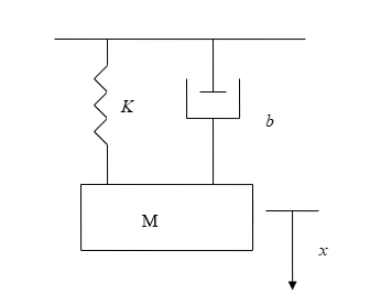
Figure 1. Spring-mass damper system
Above is the schematic diagram of a spring-mass-damper system. A block is suspended freely using a spring. As most physical systems involve damping - viscous damping, dry damping, magnetic damping, etc., a damper or dashpot is attached to account for viscous damping.
Let the mass of the block be \(M\), the spring constant be \(K\), and the damper coefficient be \(b\). If we measure displacement from the static equilibrium position, we need not consider gravitational force as it is balanced by tension in the spring at equilibrium.
Below is the free-body diagram of the block at static and dynamic equilibrium. So, the equation of motion is given by
\[Ma = F_{S} + F_{D}\;\;\;\;\;\;\;\;\;\;\;\; (1)\]
where
\[F_{S}\ \text{is the restoring force due to spring.}\]
\[F_{D}\ \text{is the damping force due to the damper.}\]
\[a\ \text{is the acceleration.}\]
The restoring force in the spring is given by
\[F_{S} = - Kx\;\;\;\;\;\;\;\;\;\;\;\; (2)\]
as the restoring force is proportional to the displacement. The damping force in the damper is given by
\[F_{D} = - bv\;\;\;\;\;\;\;\;\;\;\;\; (3)\]
as the damping force is directly proportional to velocity.
Therefore, the equation of motion can be written as
\[Ma = - Kx - bv\;\;\;\;\;\;\;\;\;\;\;\; (4)\]
At this stage, Equation (4) is a simple equation, where if we know five of the six variables, we can calculate the sixth one. However, such an expectation is not suitable. Assuming that the physical constants, \(M,\ K,\) and \(b\) are fixed and known, we are still left with three variables \(a\),\(\ v,\) and \(x\). Now, again, if we now know two of the three variables, \(a\),\(\ v,\) and \(x\), we can calculate the unknown one. However, such an expectation is still not suitable. But you recognize that
\[v = \frac{{dx}}{{dt}}\]
\[a = \frac{d^{2}x}{dt^{2}}\]
and hence from Equation (4), we get
\[M\frac{d^{2}x}{dt^{2}} = - Kx - b\frac{{dx}}{{dt}}\]
\[M\frac{d^{2}x}{dt^{2}} + b\frac{{dx}}{{dt}} + Kx = 0\;\;\;\;\;\;\;\;\;\;\;\; (5)\]
Equation (5) is an ordinary differential equation of second order and degree one. We have reduced Equation (4) from three variables to one at the expense of converting it into an ordinary differential equation. Moreover, two initial conditions, one on \(x\) and another on \(\displaystyle v = \frac{{dx}}{{dt}}\) are expected to be available.
Learning Objectives
After successful completion of this lesson, you should be able to:
1) solve the linear ordinary differential equation of first order with fixed constants by using a classical solution technique.
Introduction
In this lesson, we will revisit the classical solution technique used to solve ordinary differential equations. Knowing this technique is a prerequisite to the course.
Classical Technique
The general form of a linear ordinary differential equation with constant coefficients is given by
\[\frac{d^{n}y}{dx^{n}} + k_{n}\frac{d^{n - 1}y}{dx^{n - 1}} + ......... + k_{3}\frac{d^{2}y}{dx^{2}} + k_{2}\frac{{dy}}{{dx}} + k_{1}y = F(x)\;\;\;\;\;\;\;\;\;\;\;\; (1)\]
The general solution contains two parts
\[y = y_{H} + y_{P}\;\;\;\;\;\;\;\;\;\;\;\; (2)\]
where
\[y_{H}\ \text{is the homogeneous part of the solution and}\]
\[y_{P}\ \text{is the particular part of the solution.}\]
You can skip to the examples if you are already familiar with the theory.
Homogenous Part of the Solution
The homogeneous part of the solution \(y_{H}\) is that part of the solution that gives zero when substituted in the left-hand side of the equation. So, \(y_{H}\) is the solution of the equation
\[\frac{d^{n}y}{dx^{n}} + k_{n}\frac{d^{n - 1}y}{dx^{n - 1}} + ......... + k_{3}\frac{d^{2}y}{dx^{2}} + k_{2}\frac{{dy}}{{dx}} + k_{1}y = 0\;\;\;\;\;\;\;\;\;\;\;\; (3)\]
Equation (3) can be symbolically written as
\[D^{n}y + k_{n}D^{n - 1}y + ................. + k_{2}{Dy} + k_{1}y = 0\;\;\;\;\;\;\;\;\;\;\;\; (4)\]
\[(D^{n} + k_{n}D^{n - 1} + ................. + k_{2}D + k_{1})y = 0\;\;\;\;\;\;\;\;\;\;\;\; (5)\]
where,
\[D^{n} = \frac{d^{n}}{dx^{n}}\]
\[D^{n - 1} = \frac{d^{n - 1}}{dx^{n - 1}}.\]
\[\vdots\]
operating on \(y\) is the same as
\[(D - r_{1}),(D - r_{2}),\ (D - r_{n})\]
operating one after the other in any order, where
\[(D - r_{1}),(D - r_{2}),............,(D - r_{n})\]
are factors of
\[D^{n} + k_{n}D^{n - 1} + ............... + k_{2}D + k_{1} = 0\;\;\;\;\;\;\;\;\;\;\;\; (6)\]
To illustrate
\[(D^{2} - 3D + 2)y = 0\]
is same as
\[(D - 2)(D - 1)y = 0\]
\[(D - 1)(D - 2)y = 0\]
Therefore
\[(D^{n} + k_{n}D^{n - 1} + .................... + k_{2}D + k_{1})y = 0\;\;\;\;\;\;\;\;\;\;\;\; (7)\]
is same as
\[(D - r_{n})(D - r_{n - 1})..................(D - r_{1})y = 0\;\;\;\;\;\;\;\;\;\;\;\; (8)\]
operating one after the other in any order.
Case 1: Roots are real and distinct
The entire left-hand side becomes zero if \(\left( D - r_{1} \right)y = 0\). Therefore, the solution to \(\left( D - r_{1} \right)y = 0\) is a solution to a homogeneous equation. \(\left( D - r_{1} \right)y = 0\) is called Leibnitz’s linear differential equation of first order, and its solution is
\[\left( D - r_{1} \right)y = 0\;\;\;\;\;\;\;\;\;\;\;\; (9)\]
\[\frac{{dy}}{{dx}} = r_{1}y\;\;\;\;\;\;\;\;\;\;\;\; (10)\]
\[\frac{{dy}}{y} = r_{1}{dx}\;\;\;\;\;\;\;\;\;\;\;\; (11)\]
Integrating both sides, we get
\[\ln y = r_{1}x + c\]
\[y = ce^{r_{1}x}\;\;\;\;\;\;\;\;\;\;\;\; (12)\]
Since any of the \(n\) factors can be placed before \(y\), there are \(n\) different solutions corresponding to \(n\) different factors given by
\[C_{n}e^{r_{n}x},C_{n - 1}e^{r_{n - 1}x},..............,C_{2}e^{r_{2}x},C_{1}e^{r_{1}x}\]
where
\[r_{n,}r_{n - 1},...........,r_{2},r_{1}\ \text{are the roots of Equation (12) and}\]
\[C_{n,}C_{n - 1},......,C_{2},C_{1}\ \text{are constants.}\]
We get the general solution for a homogeneous equation by superimposing the individual Leibnitz’s solutions. Therefore
\[y_{H} = C_{1}e^{r_{1}x} + C_{2}e^{r_{2}x} + ............. + C_{n - 1}e^{r_{n - 1}x} + C_{n}e^{r_{n}x}\;\;\;\;\;\;\;\;\;\;\;\; (13)\]
Case 2: Roots are real and identical
If two roots of a homogeneous equation are equal, say \(r_{1} = r_{2}\), then
\[(D - r_{n})(D - r_{n - 1})......................(D - r_{1})(D - r_{1})y = 0\;\;\;\;\;\;\;\;\;\;\;\; (14)\]
Let’s work at
\[(D - r_{1})(D - r_{1})y = 0\;\;\;\;\;\;\;\;\;\;\;\; (15)\]
If
\[(D - r_{1})y = z\;\;\;\;\;\;\;\;\;\;\;\; (16)\]
then
\[(D - r_{1})z = 0\]
\[z = C_{2}e^{r_{1}x}\;\;\;\;\;\;\;\;\;\;\;\; (17)\]
Now substituting the solution from Equation (17) in Equation (16)
\[(D - r_{1})y = C_{2}e^{r_{1}x}\]
\[\frac{{dy}}{{dx}} - r_{1}y = C_{2}e^{r_{1}x}\]
\[e^{- r_{1}x}\frac{{dy}}{{dx}} - r_{1}e^{- r_{1}x}y = C_{2}\]
\[\frac{d(e^{- r_{1}x}y)}{{dx}} = C_{2}\]
\[d(e^{- r_{1}x}y) = C_{2}{dx}\;\;\;\;\;\;\;\;\;\;\;\; (18)\]
Integrating both sides of Equation (18), we get
\[e^{- r_{1}x}y = C_{2}x + C_{1}\]
\[y = (C_{2}x + C_{1})e^{r_{1}x}\;\;\;\;\;\;\;\;\;\;\;\; (19)\]
Therefore, the final homogeneous solution is given by
\[y_{H} = \left( C_{1} + C_{2}x \right)e^{r_{1}x} + C_{3}e^{r_{3}x} + ... + C_{n}e^{r_{n}x}\;\;\;\;\;\;\;\;\;\;\;\; (20)\]
Similarly, if \(m\) roots are identical, the solution is given by
\[y_{H} = \left( C_{1} + C_{2}x + C_{3}x^{2} + ....... + C_{m}x^{m - 1} \right)e^{r_{m}x} + C_{m + 1}e^{r_{m + 1}x} + ... + C_{n}e^{r_{n}x}\;\;\;\;\;\;\;\;\;\;\;\; (21)\]
Case 3: Roots are complex
If one pair of roots is complex, say \(r_{1} = \alpha + i\beta\) and \(r_{2} = \alpha - {i \beta }\),
where
\[i = \sqrt{- 1}\]
then
\[y_{H} = C_{1}e^{\left( \alpha + {i \beta } \right)x} + C_{2}e^{\left( \alpha - {i \beta } \right)x} + C_{3}e^{r_{3}x} + ...... + C_{n}e^{r_{n}x}\;\;\;\;\;\;\;\;\;\;\;\; (22)\]
Since
\[e^{i \beta x} = \cos\beta x + i\sin\beta x,\ \text{and}\;\;\;\;\;\;\;\;\;\;\;\; (23a)\]
\[e^{- {i \beta x}} = \cos\beta x - i\sin\beta x\;\;\;\;\;\;\;\;\;\;\;\; (23b)\]
then
\[\begin{split} y_{H} &= C_{1}e^{{\alpha x}}\left( \cos\beta x + i\sin\beta x \right) + C_{2}e^{{\alpha x}}\left( \cos\beta x - i\sin\beta x \right) + C_{3}e^{r_{3}x} + .... + C_{n}e^{r_{n}x}\\ &= \left( C_{1} + C_{2} \right)e^{{\alpha x}}\cos\beta x + i\left( C_{1} - C_{2} \right)e^{{\alpha x}}\sin\beta x + C_{3}e^{r_{3}x} + .... + C_{n}e^{r_{n}x}\\ &= e^{{\alpha x}}\left( A\cos\beta x + B\sin\beta x \right) + C_{3}e^{r_{3}x} + .... + C_{n}e^{r_{n}x}\;\;\;\;\;\;\;\;\;\;\;\; (24) \end{split}\]
where
\[A = C_{1} + C_{2}\ \text{and}\]
\[B = i(C_{1} - C_{2})\;\;\;\;\;\;\;\;\;\;\;\; (25)\]
Particular Part of the Solution
Now, let us look at how the particular part of the solution is found. Consider the general form of the ordinary differential equation
\[\left( D^{n} + k_{n}D^{n - 1} + k_{n - 1}D^{n - 2} + .......... + k_{1} \right)y = F(x)\;\;\;\;\;\;\;\;\;\;\;\; (26)\]
The particular part of the solution \(y_{P}\) is that part of the solution that gives \(F(x)\) when substituted for \(y\) in the above equation, that is,
\[\left( D^{n} + k_{n}D^{n - 1} + k_{n - 1}D^{n - 2} + ...... + k_{1} \right)y_{P} = F(x)\;\;\;\;\;\;\;\;\;\;\;\; (27)\]
Examples of what the particular part of the solution looks like are given below.
1. When
\[F(x) = e^{{ax}},\]
the particular part of the solution is of the form
\[Ae^{{ax}}.\]
We can find \(A\) by substituting
\[y_{P}\left( x \right) = Ae^{{ax}}\;\;\;\;\;\;\;\;\;\;\;\; (28)\]
in the left-hand side of the differential equation and equating coefficient of \(e^{{ax}}\).
2. When
\[F(x) = \sin{bx}\ \text{or}\ \cos{bx}.\]
the particular part of the solution is of the form
\[A\sin{bx} + B\cos{bx}.\]
We can get \({A }\)and \(B\) by substituting
\[y_{P}\left( x \right) = A\sin{bx} + B\cos{bx}\;\;\;\;\;\;\;\;\;\;\;\; (29)\]
in the left-hand side of the differential equation and equating the coefficients of \(\sin{bx}\) and/or \(\cos{bx}\).
3. When
\[X = e^{{ax}}\sin{bx}\ \text{or}\ e^{{ax}}\cos{bx},\]
the particular part of the solution is of the form
\[e^{{ax}}\left( A\sin{bx} + B\cos{bx} \right).\]
We can get \(A\) and \({B }\) by substituting
\[y_{P}\left( x \right) = e^{{ax}}(A\sin{bx} + B\cos{bx})\;\;\;\;\;\;\;\;\;\;\;\; (30)\]
in the left-hand side of the differential equation and equating coefficients of \(e^{{ax}}\sin{bx}\) and \(e^{{ax}}(A\cos{bx)}\).
The forms of the particular part of the solution for different forcing functions of ordinary differential equations are given below
| \(F(x)\) | \(y_{P}\left( x \right)\) |
|---|---|
| \(a_{0} + a_{1}x + a_{2}x^{2}\) | \(b_{0} + b_{1}x + b_{2}x^{2}\) |
| \(e^{{ax}}\) | \(Ae^{{ax}}\) |
| \(\sin{(bx)}\) | \(A\sin{(bx)} + B\cos{(bx)}\) |
| \(e^{{ax}}\sin{(bx)}\) | \(e^{{ax}}\left( A\sin{(bx)} + B\cos{(bx)} \right)\) |
| \(\cos{(bx)}\) | \(A\sin{(bx)} + B\cos{(bx)}\) |
| \(e^{{ax}}\cos{(bx)}\) | \(e^{{ax}}\left( A\sin{(bx)} + B\cos{(bx)} \right)\) |
Example 1
Solve
\[3\frac{{dy}}{{dx}} + 2y = e^{- x},\ y(0) = 5\]
Solution
The homogeneous solution for the above equation is given by
\[\left( 3D + 2 \right)y = 0\]
The characteristic equation for the above equation is given by
\[3r + 2 = 0\]
The solution to the equation is
\[r = - 0.666667\]
\[y_{H} = Ce^{- 0.666667x}\]
The particular part of the solution is of the form \(Ae^{- x}\)
\[3\frac{d\left( Ae^{- x} \right)}{{dx}} + 2Ae^{- x} = e^{- x}\]
\[- 3Ae^{- x} + 2Ae^{- x} = e^{- x}\]
\[- Ae^{- x} = e^{- x}\]
\[A = - 1\]
Hence the particular part of the solution is
\[y_{P} = - e^{- x}\]
The complete solution is given by
\[\begin{split} y &= y_{H} + y_{P}\\ &= Ce^{- 0.666667x} - e^{- x} \end{split}\]
The constant \(C\) can be obtained by using the initial condition \(y(0) = 5\)
\[y\left( 0 \right) = Ce^{- 0.666667 \times 0} - e^{- 0} = 5\]
\[C - 1 = 5\]
\[C = 6\]
The complete solution is
\[y = 6e^{- 0.666667x} - e^{- x}\]
Example 2
Solve
\[2\frac{{dy}}{{dx}} + 3y = e^{- 1.5x},\ y(0) = 5\]
Solution
The homogeneous solution for the above equation is given by
\[\left( 2D + 3 \right)y = 0\]
The characteristic equation for the above equation is given by
\[2r + 3 = 0\]
The solution to the equation is
\[r = - 1.5\]
\[y_{H} = Ce^{- 1.5x}\]
Based on the forcing function of the ordinary differential equations, the particular part of the solution is of the form \(Ae^{- 1.5x}\), but since that is part of the form of the homogeneous part of the solution, we need to choose the next independent solution, that is,
\[y_{P} = {Ax}e^{- 1.5x}\]
To find \(A\), we substitute this solution in the ordinary differential equation as
\[2\frac{d}{{dx}}({Ax}e^{- 1.5x}) + 3{Ax}e^{- 1.5x} = e^{- 1.5x}\]
\[2Ae^{- 1.5x} - 3{Ax}e^{- 1.5x} + 3{Ax}e^{- 1.5x} = e^{- 1.5x}\]
\[2Ae^{- 1.5x} = e^{- 1.5x}\]
\[A = 0.5\]
Hence the particular part of the solution is
\[y_{P} = 0.5xe^{- 1.5x}\]
The complete solution is given by
\[\begin{split} y &= y_{H} + y_{P}\\ &= Ce^{- 1.5x} + 0.5xe^{- 1.5x} \end{split}\]
The constant \(C\) is obtained by using the initial condition \(y(0) = 5\).
\[y\left( 0 \right) = Ce^{- 1.5(0)} + 0.5(0)e^{- 1.5(0)} = 5\]
\[C + 0 = 5\]
\[C = 5\]
The complete solution is
\[y = 5e^{- 1.5x} + 0.5xe^{- 1.5x}\]
Learning Objectives
After successful completion of this lesson, you should be able to:
1) solve linear ordinary differential equations of first-order with fixed constants by using classical solution techniques.
Applications
In this lesson, we revisit the classical solution technique used to solve ordinary differential equations of the second order. Knowing this technique is a prerequisite to the course.
Example 1
Solve
\[2\frac{d^{2}y}{dx^{2}} + 3\frac{{dy}}{{dx}} + 3.125y = \sin x,\ y(0) = 5,\ \frac{{dy}}{{dx}}(x = 0) = 3\]
Solution
The homogeneous equation is given by
\[(2D^{2} + 3D + 3.125)y = 0\]
The characteristic equation is
\[2r^{2} + 3r + 3.125 = 0\]
The roots of the characteristic equation are
\[\begin{split} r &= \frac{- 3 \pm \sqrt{3^{2} - 4 \times 2 \times 3.125}}{2 \times 2}\\ &= \frac{- 3 \pm \sqrt{9 - 25}}{4}\\ &= \frac{- 3 \pm \sqrt{- 16}}{4}\\ &= \frac{- 3 \pm 4i}{4}\\ &= - 0.75 \pm i \end{split}\]
Therefore the homogeneous part of the solution is given by
\[y_{H} = e^{- 0.75x}(K_{1}\cos x + K_{2}\sin x)\]
The particular part of the solution is of the form
\[y_{P} = A\sin x + B\cos x\]
\[2\frac{d^{2}}{dx^{2}}\left( A\sin x + B\cos x \right) + 3\frac{d}{{dx}}\left( A\sin x + B\cos x \right) + 3.125(A\sin x + B\cos x) = \sin x\]
\[2\frac{d}{{dx}}\left( A\cos x - B\sin x \right) + 3(A\cos x - B\sin x) + 3.125(A\sin x + B\cos x) = \sin x\]
\[2( - A\sin x - B\cos x) + 3(A\cos x - B\sin x) + 3.125(A\sin x + B\cos x) = \sin x\]
\[(1.125A - 3B)\sin x + (1.125B + 3A)\cos x = \sin x\]
Equating coefficients of \(\sin x\) and \(\cos x\) on both sides, we get
\[1.125A - 3B = 1\]
\[1.125B + 3A = 0\]
Solving the above two simultaneous linear equations, we get
\[A = 0.109589\]
\[B = - 0.292237\]
Hence
\[y_{P} = 0.109589\sin x - 0.292237\cos x\]
The complete solution is given by
\[y = e^{- 0.75x}(K_{1}\cos x + K_{2}\sin x) + (0.109589\sin x - 0.292237\cos x)\]
To find \(K_{1}\) and \(K_{2}\) we use the initial conditions
\[y(0) = 5,\ \frac{{dy}}{{dx}}(x = 0) = 3\]
From \(y(0) = 5\), we get
\[5 = e^{- 0.75(0)}(K_{1}\cos(0) + K_{2}\sin(0)) + (0.109589\sin(0) - 0.292237\cos(0))\]
\[5 = K_{1} - 0.292237\]
\[K_{1} = 5.292237\]
\[\begin{split} \frac{{dy}}{{dx}} &= - 0.75e^{- 0.75x}(K_{1}\cos x + K_{2}\sin x) + e^{- 0.75x}( - K_{1}\sin x + K_{2}\cos x)\\ & \ \ \ \ \ +0.109589\cos{x}+0.292237\sin{x} \end{split}\]
From
\[\frac{{dy}}{{dx}}(x = 0) = 3,\]
we get
\[\begin{split} 3 &= - 0.75e^{- 0.75(0)}(K_{1}\cos(0) + K_{2}\sin(0)) + \ e^{- 0.75(0)}( - K_{1}\sin(0) + K_{2}\cos(0))\\ & \ \ \ \ \ + 0.109589\cos(0) + 0.292237\sin(0) \end{split}\]
\[3 = - 0.75K_{1} + K_{2} + 0.109589\]
\[3 = - 0.75(5.292237) + K_{2} + 0.109589\]
\[K_{2} = 6.859588\]
The complete solution is
\[y = e^{- 0.75x}(5.292237\cos x + 6.859588\sin x) + 0.109589\sin x - 0.292237\cos x\]
Example 2
Solve
\[2\frac{d^{2}y}{dx^{2}} + 6\frac{{dy}}{{dx}} + 3.125y = \cos(x),\ y(0) = 5,\ \frac{{dy}}{{dx}}(x = 0) = 3\] Solution
The homogeneous part of the equations is given by
\[(2D^{2} + 6D + 3.125)y = 0\]
The characteristic equation is given by
\[2r^{2} + 6r + 3.125 = 0\]
\[\begin{split} r &= \frac{- 6 \pm \sqrt{6^{2} - 4(2)(3.125)}}{2(2)}\\ &= \frac{- 6 \pm \sqrt{36 - 25}}{4}\\ &= \frac{- 6 \pm \sqrt{11}}{4}\\ &= - 1.5 \pm 0.829156\\ &= - 0.670844, - 2.329156 \end{split}\]
Therefore, the homogeneous solution \(y_{H}\) is given by
\[y_{H} = K_{1}e^{- 0.670845x} + K_{2}e^{- 2.329156x}\]
The particular part of the solution is of the form
\[y_{P} = A\sin x + B\cos x\]
Substituting the particular part of the solution in the differential equation,
\[\begin{split} 2\frac{d^{2}}{dx^{2}}\left( A\sin x + B\cos x \right) &+ 6\frac{d}{{dx}}(A\sin x + B\cos x)\\ &+ 3.125(A\sin x + B\cos x) = \cos x \end{split}\]
\[\begin{split} 2\frac{d}{{dx}}(A\cos x - B\sin x) &+ 6(A\cos x - B\sin x)\\ &+ 3.125(A\sin x + B\cos x) = \cos x \end{split}\]
\[\begin{split} 2( - A\sin x - B\cos x) &+ 6(A\cos x - B\sin x)\\ &+ 3.125(A\sin x + B\cos x) = \cos x \end{split}\]
\[(1.125A - 6B)\sin x + (1.125B + 6A)\cos x = \cos x\]
Equating coefficients of \(\cos x\) and \(\sin x\) we get
\[1.125B + 6A = 1\]
\[1.125A - 6B = 0\]
The solution to the above two simultaneous linear equations are
\[A = 0.161006\]
\[B = 0.0301887\]
Hence the particular part of the solution is
\[y_{P} = 0.161006\sin x + 0.0301887\cos x\]
Therefore the complete solution is
\[y = y_{H} + y_{P}\]
\[y = (K_{1}e^{- 0.670845x} + K_{2}e^{- 2.329156x}) + 0.161006\sin x + 0.0301887\cos x\]
Constants \(K_{1}\) and \(K_{2}\) can be determined using initial conditions. From \(y(0) = 5\),
\[y(0) = K_{1} + K_{2} + 0.0301887 = 5\]
\[K_{1} + K_{2} = 5 - 0.0301887 = 4.969811\]
Now
\[\begin{split} \frac{dy}{dx}= &-0.670845K_1e^{-\left(0.670845\right)x}-2.329156K_2e^{-\left(2.329156\right)x}\\ &+ 0.161006\cos x - 0.0301887\sin x \end{split}\]
From
\[\frac{{dy}}{{dx}}(x = 0) = 3\]
we get
\[- 0.670845K_{1} - 2.329156K_{2} + 0.161006 = 3\]
\[0.670845K_{1} + 2.329156K_{2} = - 3 + 0.161006\]
\[0.670845K_{1} + 2.329156K_{2} = - 2.838994\]
We have two simultaneous linear equations with two unknowns
\[K_{1} + K_{2} = 4.969811\]
\[0.670845K_{1} + 2.329156K_{2} = - 2.838994\]
Solving the two simultaneous linear equations, we get
\[K_{1} = 8.692253\]
\[K_{2} = - 3.722442\]
The complete solution is
\[\begin{split} y = &(8.692253e^{- 0.670845x} - 3.722442e^{- 2.329156x})\\ &+ 0.161006\sin x + 0.0301887\cos x. \end{split}\]
Example 3
Solve
\[2\frac{d^{2}y}{dx^{2}} + 5\frac{{dy}}{{dx}} + 3.125y = e^{- x}\sin x,\ y(0) = 5,\ \frac{{dy}}{{dx}}(x = 0) = 3\]
Solution
The homogeneous equation is given by
\[(2D^{2} + 5D + 3.125)y = 0\]
The characteristic equation is given by
\[2r^{2} + 5r + 3.125 = 0\]
\[\begin{split} r &= \frac{- 5 \pm \sqrt{5^{2} - 4(2)(3.125)}}{2(2)}\\ &= \frac{- 5 \pm \sqrt{25 - 25}}{4}\\ &= \frac{- 5 \pm 0}{4}\\ &= - 1.25, - 1.25 \end{split}\]
Since roots are repeated, the homogeneous solution \(y_{H}\) is given by
\[y_{H} = (K_{1} + K_{2}x)e^{( - 1.25)x}\]
The particular part of the solution is of the form
\[y_{P} = e^{- x}(A\sin x + B\cos x)\]
Substituting the particular part of the solution in the ordinary differential equation
\[\begin{split} 2\frac{d^{2}}{dx^{2}}&{ e^{- x}(A\sin x + B\cos x)} + 5\frac{d}{{dx}}{ e^{- x}(A\sin x + B\cos x)}\\ &+3.125{e^{-x}(A\sin{x}+Bcos{x})}=e^{-x}\sin{x} \end{split}\]
\[\begin{split} &2\frac{d}{{dx}} \left\{- e^{- x}\left( A\sin x + B\cos x \right) + e^{- x}\left( A\cos x - B\sin x \right) \right\}\\ &+ 5\left\{- e^{- x}\left( A\sin x + B\cos x \right) + e^{- x}\left(A\cos x - B\sin x \right) \right\}\\ &+ 3.125e^{- x}\left( A\sin x + B\cos x \right)\end{split}\]
\[\begin{split} = e^{- x} &\sin x\ 2\{ e^{- x}(A\sin x + B\cos x) - e^{- x}(A\cos x - B\sin x) - e^{- x}(A\cos x\\ &-B\sin{x})-e^{-x}(A\sin{x}+Bcos{x})\\ &+ 5\{ - e^{- x}(A\sin x + B\cos x) + e^{- x}(A\cos x - B\sin x)\} + 3.125e^{- x}(A\sin x\\ &+ B\cos x) = e^{- x}\sin x \end{split}\]
\[- 1.875e^{- x}(A\sin x + B\cos x) + e^{- x}(A\cos x - B\sin x) = e^{- x}\sin x\]
\[- 1.875(A\sin x + B\cos x) + (A\cos x - B\sin x) = \sin x\]
\[- (1.875A + B)\sin x + (A - 1.875B)\cos x = \sin x\]
Equating coefficients of \(\cos x\) and \(\sin x\) on both sides, we get
\[A - 1.875B = 0\]
\[1.875A + B = - 1\]
Solving the above two simultaneous linear equations, we get
\[A = - 0.415224\ \text{and}\]
\[B = - 0.221453\]
Hence,
\[y_{P} = - e^{- x}(0.415224\sin x + 0.221453\cos x)\]
Therefore the complete solution is given by
\[y = y_{H} + y_{P}\]
\[y = (K_{1} + xK_{2})e^{- 1.25x} - e^{- x}(0.415224\sin x + 0.221453\cos x)\]
Constants \(K_{1}\) and \(K_{2}\) can be determined using initial conditions,
From \(y(0) = 5,\) we get
\[K_{1} - 0.221453 = 5\]
\[K_{1} = 5.221453\]
Now
\[\begin{split} \frac{dy}{dx}= &-1.25K_1e^{-1.25x}-1.25K_2xe^{-1.25x}+K_2e^{-1.25x}-\\ &e^{- x}(0.415224\cos x - 0.221453\sin x) + e^{- x}(0.415224\sin x + 0.221453\cos x) \end{split}\]
From \(\displaystyle \frac{{dy}}{{dx}}(0) = 3,\) we get
\[\begin{split} &- 1.25K_{1}e^{- 1.25(0)} - 1.25K_{2}(0)e^{- 1.25(0)} + K_{2}e^{- 1.25(0)}\\ &-e^0(0.415224\cos(0)-0.221453\sin(0))+e^0(0.415224\sin(0)+0.221453\cos(0)=3 \end{split}\]
\[- 1.25K_{1} + K_{2} + 0.221453 - 0.415224 = 3\]
\[- 1.25K_{1} + K_{2} = 3.193771\]
\[- 1.25(5.221453) + K_{2} = 3.193771\]
\[K_{2} = 9.720582\]
Substituting
\[K_{1} = 5.221453\ \text{and}\]
\[K_{2} = 9.720582\]
in the solution, we get
\[y = (5.221453 + 9.720582x)e^{- 1.25x} - e^{- x}(0.415224\sin x + 0.221453\cos x)\]
Learning Objectives
After successful completion of this lesson, you should be able to:
1) recall the two parts of the fundamental theorem of calculus
2) verify finding an exact integral using the exact solution of a first-order ordinary differential equation
Introduction
In this lesson, we recall the two parts of the fundamental theorem of calculus (sometimes called the first and second fundamental theorems of calculus) to be able to show that the solution to a definite integral
\[\int_{a}^{b}{f(x)dx}\]
can be posed as a solution to an ordinary differential equation. This ability to represent a definite integral as an ordinary differential equation plays a prominent role in showing how we can use numerical methods of ordinary differential equations to conduct numerical integration.
The first part of the fundamental theorem of calculus states that if \(f(x)\) is a real-valued and continuous function in the open interval D, and a is a point in the interval D, and if
\[F(x) = \int_{a}^{x}{f(t)dt}\;\;\;\;\;\;\;\;\;\;\;\; (1)\]
then
\[F^{\prime}(x) = f(x)\;\;\;\;\;\;\;\;\;\;\;\; (2)\]
at each point in D.
The second part of the fundamental theorem of calculus states that if \(f(x)\) is a real-valued function in the interval \(\lbrack a,b\rbrack\), and \(F(x)\) is the antiderivative of \(f(x)\) in \(\lbrack a,b\rbrack\), then
\[\int_{a}^{b}{f(x)dx} = F\left( b \right) - F\left( a \right)\;\;\;\;\;\;\;\;\;\;\;\; (3)\]
Hence we can write equation (1) as
\[\frac{{dF}}{{dx}} = f(x)\;\;\;\;\;\;\;\;\;\;\;\; (4)\]
and if we assume \(F\left( a \right) = 0\), then from Equation (3)
\[\int_{a}^{b}{f(x)dx} = F(b)\;\;\;\;\;\;\;\;\;\;\;\; (5)\]
So we can pose the value of \(\int_{a}^{b}{f(x)dx}\) as solving Equation (4) for \(F(b)\) with \(F\left( a \right) = 0\) as the initial condition. We use the example below to illustrate the equivalency.
Example 1
Let us suppose you are asked to find
\[\int_{3}^{9}{5x^{2}{dx}}\;\;\;\;\;\;\;\;\;\;\;\; (E1.1)\]
The exact integral using integral calculus is given as
\[\begin{split} \int_{3}^{9}{5x^{2}{dx}} &= \ \left\lbrack \frac{5x^{3}}{3} \right\rbrack_{3}^{9}\\ &= \frac{5{(9)}^{3}}{3} - \frac{5{(3)}^{3}}{3}\\ &= \ 1215 - 45\\ &= 1170\;\;\;\;\;\;\;\;\;\;\;\; (E1.2) \end{split}\]
Now, if one poses an ordinary differential equation
\[\frac{{dy}}{{dx}} = \ 5x^{2}\ ,\ y\left( 3 \right) = 0\;\;\;\;\;\;\;\;\;\;\;\; (E1.3)\]
then the solution using the classical solution technique is as follows
\[y = \ y_{H} + y_{P}\;\;\;\;\;\;\;\;\;\;\;\; (E1.4)\]
The homogeneous part of the solution, \(y_{H}\) is found by using the characteristic equation
\[m = 0\]
to give
\[\begin{split} y_{H} &= Ke^{0x}\\ &= K\;\;\;\;\;\;\;\;\;\;\;\; (E1.5) \end{split}\]
The particular part of the solution would be of the form of \(Ax^{2} + Bx + C\), but since the constant \(C\) is part of the homogeneous part of the solution, \(y_{H} = K\), we need to use the next independent solution.
\[\begin{split} y_{P} &= x\left( Ax^{2} + Bx + C \right)\\ &= Ax^{3} + Bx^{2} + Cx\;\;\;\;\;\;\;\;\;\;\;\; (E1.6) \end{split}\]
By substituting \(y_{P}\) in the ordinary differential equation, we get
\[\frac{d}{{dx}}\left( Ax^{3} + Bx^{2} + Cx \right) = 5x^{2}\]
\[3Ax^{2} + 2Bx + C = 5x^{2} + 0x + 0\]
giving
\[3A = 5\]
\[2B = 0\]
\[C = 0\]
and hence
\[A = \frac{5}{3}\]
\[B = 0\]
\[C = 0\]
So Equation (E1.6) gives
\[y_{P} = \frac{5}{3}x^{3}\;\;\;\;\;\;\;\;\;\;\;\; (E1.7)\]
The complete solution from Equation (E1.4) is
\[\begin{split} y &= \ y_{H} + y_{P}\\ &= \ K + \frac{5}{3}x^{3}\;\;\;\;\;\;\;\;\;\;\;\; (E1.8) \end{split}\]
To find \(K\), use the initial condition,
\[y(3) = 0\]
then from Equation (E1.8), we get
\[K + \frac{5}{3}{(3)}^{3} = 0\]
\[K + 45 = 0\]
\[K = - 45\]
Hence the solution by rewriting Equation (E1.8) is
\[y = \ - 45 + \frac{5}{3}x^{3}\;\;\;\;\;\;\;\;\;\;\;\; (E1.9)\]
From Equation (E1.9)
\[\begin{split} y(9) &= \ - 45 + \frac{5}{3}{(9)}^{3}\\ &= \ 1170 \;\;\;\;\;\;\;\;\;\;\;\; (E1.10) \end{split}\]
We could have chosen \(y\left( 3 \right)\) to be any finite number and the value \(y\left( 9 \right) - y\left( 3 \right)\) would still turn out to be \(1170\).
Why do these values from Equations (E1.2) and (E1.10), one being an integral and another being the solution of an ordinary differential equation, turn out to be the same value \(1170\). It is not a coincidence. It is because of the second fundamental theorem of calculus, and it states
\[\frac{d}{{dx}}\int_{a}^{x}{f\left( t \right)dt = f(x)}\;\;\;\;\;\;\;\;\;\;\;\; (E1.11)\]
Choosing
\[f\left( t \right) = 5t^{2}\ \text{and}\ a = 3\]
\[\frac{d}{{dx}}\int_{3}^{x}{5t^{2}\ dt = 5x^{2}\ }\;\;\;\;\;\;\;\;\;\;\;\; (E1.12)\]
Calling
\[y\left( x \right) = \int_{3}^{x}{5t^{2}\ {dt}\ }\]
\[\frac{{dy}}{{dx}} = 5x^{2}\]
By posing the ordinary differential equation as
\[\frac{{dy}}{{dx}} = 5x^{2},\ y(3) = 0\;\;\;\;\;\;\;\;\;\;\;\; (E1.13)\]
and finding\(\ y(9)\), we have
\[y\left( 3 \right) = \int_{3}^{3}{5t^{2}\ dt = 0\ }\]
\[y\left( 9 \right) = \int_{3}^{9}{5t^{2}\ {dt}}\]
Hence solving
\[\frac{{dy}}{{dx}} = 5x^{2},\ y(3) = 0\]
for \(y\left( 9 \right)\) is the value of the integral
\[\int_{3}^{9}{5t^{2}\ {dt}.\ }\]
Learning Objectives
After successful completion of this lesson, you should be able to:
1) Find the exact solution of ordinary differential equations by using Laplace transforms
Introduction
If \(y = f(x)\) is defined at all positive values of \(x\), the Laplace transform denoted by \(Y(s)\) is given by
\[Y(s) = L\{ f(x)\} = \int_{0}^{\infty}e^{- {sx}}f(x)dx\ \ \ (35)\]
where \(s\) is a parameter, which can be a real or complex number. We can get back \(f(x)\) by taking the inverse Laplace transform of \(Y(s)\).
\[L^{- 1}\{ Y(s)\} = f(x)\ \ \ (36)\]
Laplace transforms are highly useful in solving differential equations. They give the solution directly without the necessity of evaluating arbitrary constants separately.
The following are Laplace transforms of some elementary functions
\[L(1) = \frac{1}{s}\] \[L(x^{n}) = \frac{n!}{s^{n + 1}},\ \text{where}\ n = 0,1,2,3...\] \[L(e^{{ax}}) = \frac{1}{s - a}\] \[L(\sin ax) = \frac{a}{s^{2} + a^{2}}\] \[L(\cos ax) = \frac{s}{s^{2} + a^{2}}\] \[L({\sinh}\ ax) = \frac{a}{s^{2} - a^{2}}\] \[L({\cosh}\ ax) = \frac{s}{s^{2} - a^{2}}\ \ \ (37)\]
The following are the inverse Laplace transforms of some common functions
\[L^{- 1}\left( \frac{1}{s} \right) = 1\] \[L^{- 1}\left( \frac{1}{s - a} \right) = e^{{ax}}\] \[L^{- 1}\left( \frac{1}{s^{n}} \right) = \frac{x^{n - 1}}{\left( n - 1 \right)!},\ \text{where}\ n = 1,2,3......\] \[L^{- 1}\left( \frac{1}{\left( s - a \right)^{n}} \right) = \frac{e^{{ax}}x^{n - 1}}{\left( n - 1 \right)!}\] \[L^{- 1}\left( \frac{1}{s^{2} + a^{2}} \right) = \frac{1}{a}\sin ax\] \[L^{- 1}\left( \frac{s}{s^{2} + a^{2}} \right) = \cos ax\] \[L^{- 1}\left( \frac{1}{s^{2} - a^{2}} \right) = \frac{1}{a}{\sinh}\ ax\] \[L^{- 1}\left( \frac{s}{s^{2} - a^{2}} \right) = {\cosh}\ at\] \[L^{- 1}\left( \frac{1}{\left( s - a \right)^{2} + b^{2}} \right) = \frac{1}{b}e^{{ax}}\sin bx\] \[L^{- 1}\left( \frac{s - a}{\left( s - a \right)^{2} + b^{2}} \right) = e^{{ax}}\cos bx\] \[L^{- 1}\left( \frac{s}{\left( s^{2} + a^{2} \right)^{2}} \right) = \frac{1}{2a}x\sin ax\ \ \ (38)\]
Properties of Laplace transforms
Linear property
If \(a,\ b,\ c\) are constants and \(f(x),\ g(x),\) and \(h(x)\) are functions of \(x\) then
\[L\lbrack af(x) + bg(x) + ch(x)\rbrack = aL(f(x)) + bL(g(x)) + cL(h(x))\ \ \ (39)\]
Shifting property
If
\[L\{ f(x)\} = Y(s)\ \ \ (40)\]
then
\[L\{ e^{{at}}f(x)\} = Y(s - a)\ \ \ (41)\]
Using shifting property we get
\[L\left( e^{{ax}}x^{n} \right) = \frac{n!}{\left( s - a \right)^{n + 1}},\ n \geq 0\] \[L\left( e^{{ax}}\sin bx \right) = \frac{b}{\left( s - a \right)^{2} + b^{2}}\] \[L\left( e^{{ax}}\cos bx \right) = \frac{s - a}{\left( s - a \right)^{2} + b^{2}}\] \[L\left( e^{{ax}}\sinh bx \right) = \frac{b}{\left( s - a \right)^{2} - b^{2}}\] \[L\left( e^{{ax}}\cosh bx \right) = \frac{s - a}{\left( s - a \right)^{2} - b^{2}}\ \ \ (42)\]
Scaling property
If
\[L\{ f(x)\} = Y(s)\ \ \ (43)\]
then
\[L\{ f(ax)\} = \frac{1}{a}Y\left( \frac{s}{a} \right)\ \ \ (44)\]
Laplace transforms of derivatives
If the first \(n\) derivatives of \(f(x)\) are continuous, then
\[L\{ f^{n}(x)\} = \int_{0}^{\infty}{e^{- {sx}}f^{n}(x)dx}\ \ \ (45)\]
Using integration by parts, we get
\[\begin{split} \int_{0}^{\infty}e^{- {sx}}f^{n}(x)dx &= \begin{bmatrix} \ e^{- {sx}}f^{n - 1}(x) - ( - s)e^{- {sx}}f^{n - 2}(x) \\ \ \ \ \ + ( - s)^{2}e^{- {sx}}f^{n - 3}(x) + ...... + ( - 1)^{n - 1}( - s)^{n - 1}e^{- {sx}}f(x) \\ \end{bmatrix}_{0}^{\infty}\\ &\ \ \ \ +(-1)^{n}(-s)^{n} \int_{0}^{\infty} e^{-s x} f(x) d x \\ &= - f^{n - 1}\left( 0 \right) - sf^{n - 2}\left( 0 \right) - s^{2}f^{n - 3}\left( 0 \right) - ........... - s^{n - 1}f\left( 0 \right) +\\ & \ \ \ \ \ \ \ \ s^{n}\int_{0}^{\infty}{e^{- {sx}}f(x)dx}\\ &= s^{n}Y(s) - f^{n - 1}(0) - sf^{n - 2}(0) - s^{2}f^{n - 3}(0) - ........ - s^{n - 1}f(0)\ \ \ (46) \end{split}\]
Laplace transform technique to solve ordinary differential equations
The following are steps to solve ordinary differential equations using the Laplace transform method
(A) Take the Laplace transform of both sides of ordinary differential equations.
(B) Express \(Y(s)\) as a function of \(s\).
(C) Take the inverse Laplace transform on both sides to get the solution.
Let us solve Examples 1 through 4 using the Laplace transform method.
Example 1
Solve
\[3\frac{{dy}}{{dx}} + 2y = e^{- x},\ y(0) = 5\]
Solution
Taking the Laplace transform of both sides, we get
\[\begin{split} &L\left( 3\frac{{dy}}{{dx}} + 2y \right) = L\left( e^{- x} \right)\\ &3\lbrack sY(s) - y(0)\rbrack + 2Y(s) = \frac{1}{s + 1} \end{split}\]
Using the initial condition, \(y(0) = 5\) we get
\[3\lbrack sY(s) - 5\rbrack + 2Y(s) = \frac{1}{s + 1}\] \[(3s + 2)Y(s) = \frac{1}{s + 1} + 15\] \[(3s + 2)Y(s) = \frac{15s + 16}{s + 1}\] \[Y(s) = \frac{15s + 16}{(s + 1)(3s + 2)}\]
Writing the expression for \(Y(s)\) in terms of partial fractions
\[\frac{15s + 16}{(s + 1)(3s + 2)} = \frac{A}{s + 1} + \frac{B}{3s + 2}\] \[\frac{15s + 16}{(s + 1)(3s + 2)} = \frac{3As + 2A + Bs + B}{(s + 1)(3s + 2)}\] \[15s + 16 = 3As + 2A + Bs + B\]
Equating coefficients of \(s^{1}\) and \(s^{0}\) gives
\[3A + B = 15\]
\[2A + B = 16\]
The solution to the above two simultaneous linear equations is
\[A = - 1\] \[B = 18\] \[\begin{split} Y(s) &= \frac{- 1}{s + 1} + \frac{18}{3s + 2}\\ &= \frac{- 1}{s + 1} + \frac{6}{s + 0.666667}\end{split}\]
Taking the inverse Laplace transform on both sides
\[L^{- 1}\{ Y(s)\} = L^{- 1}\left( \frac{- 1}{s + 1} \right) + L^{- 1}\left( \frac{6}{s + 0.666667} \right)\]
Since
\[L^{- 1}\left( \frac{1}{s + a} \right) = e^{- {at}}\]
The solution is given by
\[y(x) = - e^{- x} + 6e^{- 0.666667x}\]
Example 2
Solve
\[2\frac{{dy}}{{dx}} + 3y = e^{- 1.5x},\ y(0) = 5\] Solution
Taking the Laplace transform of both sides, we get
\[L\left( 2\frac{{dy}}{{dx}} + 3y \right) = L\left( e^{- 1.5x} \right)\] \[2\lbrack sY(s) - y(0)\rbrack + 3Y(s) = \frac{1}{s + 1.5}\]
Using the initial condition \(y(0) = 5\), we get
\[2\lbrack sY(s) - 5\rbrack + 3Y(s) = \frac{1}{s + 1.5}\] \[(2s + 3)Y(s) = \frac{1}{s + 1.5} + 10\] \[(2s + 3)Y(s) = \frac{10s + 16}{s + 1.5}\]
\[\begin{split} Y(s) &= \frac{10s + 16}{(s + 1.5)(2s + 3)}\\ &= \frac{10s + 16}{2(s + 1.5)(s + 1.5)}\\ &= \frac{10s + 16}{2(s + 1.5)^{2}}\\ &= \frac{5s + 8}{(s + 1.5)^{2}} \end{split}\]
Writing the expression for \(Y(s)\) in terms of partial fractions
\[\frac{5s + 8}{(s + 1.5)^{2}} = \frac{A}{s + 1.5} + \frac{B}{(s + 1.5)^{2}}\] \[\frac{5s + 8}{(s + 1.5)^{2}} = \frac{As + 1.5A + B}{(s + 1.5)^{2}}\] \[5s + 8 = As + 1.5A + B\]
Equating coefficients of \(s^{1}\) and \(s^{0}\) gives
\[A = 5\] \[1.5A + B = 8\]
The solution to the above two simultaneous linear equations is
\[A = 5\] \[B = 0.5\] \[Y(s) = \frac{5}{s + 1.5} + \frac{0.5}{(s + 1.5)^{2}}\]
Taking the inverse Laplace transform on both sides
\[L^{- 1}\{ Y(s)\} = L^{- 1}\left( \frac{5}{s + 1.5} \right) + L^{- 1}\left( \frac{0.5}{(s + 1.5)^{2}} \right)\]
Since
\[L^{- 1}\left( \frac{1}{s + a} \right) = e^{- ax}\ \text{and}\ L^{- 1}\left( \frac{1}{(s + a)^{2}} \right) = xe^{- {ax}}\]
The solution is given by
\[y(x) = 5e^{- 1.5x} + 0.5xe^{- 1.5x}\]
Example 3
Solve
\[2\frac{d^{2}y}{dx^{2}} + 3\frac{{dy}}{{dx}} + 3.125y = \sin x,\ y(0) = 5,\ \frac{{dy}}{{dx}}(x = 0) = 3\] Solution
Taking the Laplace transform of both sides
\[L\left( 2\frac{d^{2}y}{dx^{2}} + 3\frac{{dy}}{{dx}} + 3.125y \right) = L\left( \sin x \right)\]
and knowing
\[L\left( \frac{d^{2}y}{dx^{2}} \right) = s^{2}Y\left( s \right) - {sy}\left( 0 \right) - \frac{{dy}}{{dx}}\left( x = 0 \right)\] \[L\left( \frac{{dy}}{{dx}} \right) = sY\left( s \right) - y\left( 0 \right)\] \[L(\sin x) = \frac{1}{s^{2} + 1}\]
we get
\[2\left\lbrack s^{2}Y(s) - sy(0) - \frac{{dy}}{{dx}}(x = 0) \right\rbrack + 3\left\lbrack sY(s) - y(0) \right\rbrack + 3.125Y(s) = \frac{1}{s^{2} + 1}\] \[2\left[s^{2} Y(s)-5 s-3\right]+3[s Y(s)-5]+3.125 Y(s)=\frac{1}{s^{2}+1}\] \[[s(2 s+3)+3.125] Y(s)-10s-21 = \frac{1}{s^{2}+1}\] \[\left\lbrack s\left( 2s + 3 \right) + 3.125 \right\rbrack Y(s) = \frac{1}{s^{2} + 1} + 10s + 21\] \[\left\lbrack 2s^{2} + 3s + 3.125 \right\rbrack Y(s) = \frac{22 + 10s^{3} + 10s + 21s^{2}}{(s^{2} + 1)}\] \[Y(s) = \frac{10s^{3} + 21s^{2} + 10s + 22}{\left( s^{2} + 1 \right)\left( 2s^{2} + 3s + 3.125 \right)}\]
Writing the expression for \(Y(s)\) in terms of partial fractions
\[\frac{As + B}{\left( 2s^{2} + 3s + 3.125 \right)} + \frac{Cs + D}{\left( s^{2} + 1 \right)} = \frac{10s^{3} + 21s^{2} + 10s + 22}{\left( s^{2} + 1 \right)\left( 2s^{2} + 3s + 3.125 \right)}\] \[\begin{split} &\frac{As^{3} + As + Bs^{2} + B + 2Cs^{3} + 3Cs^{2} + 3.125Cs + 2Ds^{2} + 3Ds + 3.125D}{\left( 2s^{2} + 3s + 3.125 \right)\left( s^{2} + 1 \right)}\\ &= \frac{10s^{3} + 21s^{2} + 10s + 22}{\left( s^{2} + 1 \right)\left( 2s^{2} + 3s + 3.125 \right)}\end{split}\] \[\begin{split} &\frac{\left(A+2C\right)s^3+\left(B+3C+2D\right)s^2+\left(A+3.125C+3D\right)s+\left(B+3.125D\right)}{\left(s^2+1\right)\left(2s^2+3s+3.125\right)}\\ &= \frac{10s^{3} + 21s^{2} + 10s + 22}{\left( s^{2} + 1 \right)\left( 2s^{2} + 3s + 3.125 \right)} \end{split}\]
Equating terms of \(s^{3}\), \(\ s^{2},\ s^{1}\) and \(s^{0}\) gives gives four simultaneous linear equations
\[A + 2C = 10\] \[B + 3C + 2D = 21\] \[A + 3.125C + 3D = 10\] \[B + 3.125D = 22\]
The solution to the above four simultaneous linear equations is
\[A = 10.584474\] \[B = 21.657534\] \[C = - 0.292237\] \[D = 0.109589\]
Hence
\[Y(s) = \frac{10.584474s + 21.657534}{2s^{2} + 3s + 3.125} + \frac{- 0.292237s + 0.109589}{s^{2} + 1}\]
\[\left( 2s^{2} + 3s + 3.125 \right) = 2\{(s^{2} + 1.5s + 0.5625) + 1\} = 2\{(s + 0.75)^{2} + 1\}\]
\[\begin{split} Y(s) &= \frac{10.584474(s + 0.75) + 13.719179}{2\{(s + 0.75)^{2} + 1\}} + \frac{- 0.292237s + 0.109589}{s^{2} + 1}\\ &= \frac{5.292237(s + 0.75)}{\{(s + 0.75)^{2} + 1\}} + \frac{6.859589}{\{(s + 0.75)^{2} + 1\}} - \frac{0.292237s}{(s^{2} + 1)} + \frac{0.109589}{(s^{2} + 1)} \end{split}\] \[L^{-1}{Y(s)}=5.292237L^{-1}\left(\frac{s+0.75}{{(s+0.75)^2+1}}\right)+6.859589L^{-1}\left(\frac{1}{{(s+0.75)^2+1}}\right) \] Taking the inverse Laplace transform of both sides
\[\begin{split} L^{- 1}\left\{ Y\left( s \right) \right\} &= L^{- 1}\left( \frac{5.292237\left( s + 0.75 \right)}{\{(s + 0.75)^{2} + 1\}} \right) + L^{- 1}\left( \frac{6.859589}{\{(s + 0.75)^{2} + 1} \right) - L^{- 1}\left( \frac{0.292237s}{s^{2} + 1} \right) +\\ & \ \ \ \ L^{- 1}\left( \frac{0.109589}{s^{2} + 1} \right)\end{split}\] \[\begin{split} L^{-1}{Y(s)} &= 5.292237L^{-1}\left(\frac{s+0.75}{{(s+0.75)^2+1}}\right)+6.859589L^{-1}\left(\frac{1}{{(s+0.75)^2+1}}\right) \\& \ \ \ \ - 0.292237L^{- 1}\left( \frac{s}{s^{2} + 1} \right) + 0.109589L^{- 1}\left( \frac{1}{s^{2} + 1} \right) \end{split}\]
Since
\[L^{- 1}\left( \frac{s + a}{\left( s + a \right)^{2} + b^{2}} \right) = e^{- {ax}}\cos bx\] \[L^{- 1}\left( \frac{b}{\left( s + a \right)^{2} + b^{2}} \right) = e^{- {ax}}\sin bx\] \[L^{- 1}\left( \frac{1}{s^{2} + a^{2}} \right) = \sin ax\] \[L^{- 1}\left( \frac{s}{s^{2} + a^{2}} \right) = \cos ax\]
The complete solution is
\[ \begin{split} y(x) &= 5.292237e^{-0.75x}cos{x}+6.8595859e^{-0.75x}sin{x}\\& \ \ \ \ - 0.292237\cos x + 0.109589\sin x\\ &= e^{- 0.75x}\left( 5.292237\cos x + 6.859589\sin x \right) - 0.292237\cos x + 0.109589\sin x \end{split}\]
Example 4
Solve
\[2\frac{d^{2}y}{dx^{2}} + 6\frac{{dy}}{{dx}} + 3.125y = \cos x,\ y(0) = 5, \ \frac{{dy}}{{dx}}(x = 0) = 3\] Solution
Taking the Laplace transform of both sides
\[L\left( 2\frac{d^{2}y}{dx^{2}} + 6\frac{{dy}}{{dx}} + 3.125y \right) = L\left( \cos x \right)\]
and knowing
\[L\left( \frac{d^{2}y}{dx^{2}} \right) = s^{2}Y\left( s \right) - {sy}\left( 0 \right) - \frac{{dy}}{{dx}}\left( x = 0 \right)\] \[L\left( \frac{{dy}}{{dx}} \right) = sY\left( s \right) - y\left( 0 \right)\] \[L(\cos x) = \frac{s}{s^{2} + 1}\]
we get
\[2\left\lbrack s^{2}Y(s) - sy(0) - \frac{{dy}}{{dx}}(x = 0) \right\rbrack + 6\left\lbrack sY(s) - y(0) \right\rbrack + 3.125Y(s) = \frac{s}{s^{2} + 1}\] \[2\left\lbrack s^{2}Y(s) - 5s - 3 \right\rbrack + 6\left\lbrack sY(s) - 5 \right\rbrack + 3.125Y(s) = \frac{s}{s^{2} + 1}\] \[\left\lbrack s(2s + 6) + 3.125 \right\rbrack Y(s) = \frac{s}{s^{2} + 1} + 10s + 36\] \[\left\lbrack 2s^{2} + 6s + 3.125 \right\rbrack Y(s) = \frac{36 + 10s^{3} + 11s + 36s^{2}}{s^{2} + 1}\] \[Y(s) = \frac{10s^{3} + 36s^{2} + 11s + 36}{\left( s^{2} + 1 \right)\left( 2s^{2} + 6s + 3.125 \right)}\]
Writing the expression for \(Y(s)\) in terms of partial fractions
\[\frac{As + B}{\left( 2s^{2} + 6s + 3.125 \right)} + \frac{Cs + D}{\left( s^{2} + 1 \right)}\ = \frac{10s^{3} + 36s^{2} + 11s + 36}{\left( s^{2} + 1 \right)\left( 2s^{2} + 6s + 3.125 \right)}\] \[\begin{split} &\frac{As^3+As+Bs^2+B+2Cs^3+6Cs^2+3.125Cs+2Ds^2+6Ds+3.125D}{\left(2s^2+6s+3.125\right)\left(s^2+1\right)}\\ &= \frac{10s^{3} + 36s^{2} + 11s + 36}{\left( s^{2} + 1 \right)\left( 2s^{2} + 6s + 3.125 \right)}\end{split}\] \[\begin{split} &\frac{\left(A+2C\right)s^3+\left(B+6C+2D\right)s^2+\left(A+3.125C+6D\right)s+\left(B+3.125D\right)}{\left(s^2+1\right)\left(2s^2+6s+3.125\right)}\\ &= \frac{10s^{3} + 36s^{2} + 11s + 36}{\left( s^{2} + 1 \right)\left( 2s^{2} + 6s + 3.125 \right)}\end{split}\]
Equating terms of \(s^{3}\),\(\ s^{2},\ s^{1}\) and \(s^{0}\) gives
\[A + 2C = 10\] \[B + 6C + 2D = 36\] \[A + 3.125C + 6D = 11\]
\[B + 3.125D = 36\]
The solution to the above four simultaneous linear equations is
\[A = 9.939622\] \[B = 35.496855\] \[C = 0.0301886\] \[D = 0.161006\]
Then
\[Y(s) = \frac{9.939622s + 35.496855}{2s^{2} + 6s + 3.125} + \frac{0.0301886s + 0.161006}{s^{2} + 1}\]
\[\left( 2s^{2} + 6s + 3.125 \right) = 2\{(s^{2} + 3s + 2.25) - 0.6875\} = 2\{(s + 1.5)^{2} - 0.829156^{2}\}\]
\[\begin{split} Y(s) &= \frac{9.939622(s + 1.5) + 20.587422}{2\{(s + 1.5)^{2} - 0.829156^{2}\}} + \frac{0.0301886s + 0.161006}{s^{2} + 1}\\ &=\frac{4.969811(s+1.5)}{{(s+1.5)^2-0.829156^2}}+\frac{10.293711}{{(s+1.5)^2-0.829156^2}}\\ & \ \ \ \ + \frac{0.0301886s}{s^{2} + 1} + \frac{0.161006}{s^{2} + 1} \end{split}\]
Taking the inverse Laplace transform on both sides
\[\begin{split} L^{-1}{Y(s)} &= L^{-1}\left(\frac{4.969811(s+1.5)}{{(s+1.5)^2-0.829156^2}}\right)+L^{-1}\left(\frac{10.293711}{(s+1.5)^2-0.829156^2}\right)\\ &\ \ \ \ + L^{- 1}\left( \frac{0.0301886s}{s^{2} + 1} \right) + L^{- 1}\left( \frac{0.161006}{s^{2} + 1} \right)\\ &= 4.969811L^{- 1}\left( \frac{(s + 1.5)}{(s + 1.5)^{2} - 0.829156^{2}} \right) + 10.293711L^{- 1}\left( \frac{1}{(s + 1.5)^{2} - 0.829156^{2}} \right)\\ &\ \ \ \ + 0.0301886L^{- 1}\left( \frac{s}{(s^{2} + 1)} \right) + 0.161006L^{- 1}\left( \frac{1}{(s^{2} + 1)} \right) \end{split}\]
Since
\[L^{- 1}\left( \frac{s + a}{\left( s + a \right)^{2} - b^{2}} \right) = e^{- {ax}}{\cosh}\ bx\] \[L^{- 1}\left( \frac{1}{\left( s + a \right)^{2} - b^{2}} \right) = \frac{1}{b}e^{- {ax}}{\sinh}\ bx\] \[L^{- 1}\left( \frac{1}{s^{2} + a^{2}} \right) = \frac{1}{a}\sin ax\] \[L^{- 1}\left( \frac{s}{s^{2} + a^{2}} \right) = \cos ax\]
The complete solution is
\[\begin{split} y(x)&= 4.969811e^{- 1.5x}\cosh(0.829156x) + \frac{10.293711}{0.829156}e^{- 1.5x}\sinh(0.829156x)\\ & \ \ \ \ + 0.0301886\cos x + 0.161006\sin x\\ &=e^{-1.5x}\left(4.969811\left(\frac{e^{0.829156x}+e^{-0.829156x}}{2}\right)+ 12.414685\ \left(\frac{e^{0.829156x}-e^{-0.829156x}}{2}\right)\right)\\ & \ \ \ \ +0.030188\cos{x}+0.161006\sin{x} \\ &= e^{- 1.5x}\left( 8.692248e^{0.829156x} - 3.722437e^{- 0.829156x} \right) + 0.0301886\cos x \\ & \ \ \ \ + 0.161006\sin x \end{split}\]
Example 5
Solve
\[2\frac{d^{2}y}{dx^{2}} + 5\frac{{dy}}{{dx}} + 3.125y = e^{- x}\sin x,\ y(0) = 5,{\ \ }\frac{{dy}}{{dx}}(x = 0) = 3\]
Solution
Taking the Laplace transform of both sides
\[L\left( 2\frac{d^{2}y}{dx^{2}} + 5\frac{{dy}}{{dx}} + 3.125y \right) = L\left( e^{- x}\sin x \right)\]
knowing
\[L\left( \frac{d^{2}y}{dx^{2}} \right)= s^{2}Y\left( s \right) - {sy}\left( 0 \right) - \frac{{dy}}{{dx}}\left( x = 0 \right)\] \[L\left( \frac{{dy}}{{dx}} \right) = sY\left( s \right) - y\left( 0 \right)\] \[L(e^{- x}\sin x) = \frac{1}{(s + 1)^{2} + 1}\]
we get
\[2\left[s^{2} Y(s)-s y(0)-\frac{d y}{d x}(x=0)\right]+5[s Y(s)-y(0)]+3.125 Y(s)=\frac{1}{(s+1)^{2}+1}\] \[2\left[s^{2} Y(s)-5 s-3\right]+5[s Y(s)-5]+3.125 Y(s)=\frac{1}{(s+1)^{2}+1}\] \[\left\lbrack s\left( 2s + 5 \right) + 3.125 \right\rbrack Y(s) - 10s - 31 = \frac{1}{(s + 1)^{2} + 1}\] \[\left\lbrack s(2s + 5) + 3.125 \right\rbrack Y(s) = \frac{1}{(s + 1)^{2} + 1} + 10s + 31\] \[\left\lbrack 2s^{2} + 5s + 3.125 \right\rbrack Y(s) = \frac{63 + 10s^{3} + 82s + 51s^{2}}{s^{2} + 2s + 2}\] \[Y(s) = \frac{10s^{3} + 51s^{2} + 82s + 63}{\left( s^{2} + 2s + 2 \right)\left( 2s^{2} + 5s + 3.125 \right)} \]
Writing the expression for \(Y(s)\) in terms of partial fractions
\[\frac{As + B}{2s^{2} + 5s + 3.125} + \frac{Cs + D}{s^{2} + 2s + 2} = \frac{10s^{3} + 51s^{2} + 82s + 63}{\left( s^{2} + 2s + 2 \right)\left( 2s^{2} + 5s + 3.125 \right)}\] \[\begin{split} &\frac{2Cs^{3} + 5Cs^{2} + 3.125Cs + 2Ds^{2} + 5Ds + 3.125D + As^{3} + 2As^{2} + 2As + Bs^{2} + 2Bs + 2B}{\left( 2s^{2} + 5s + 3.125 \right)\left( s^{2} + 2s + 2 \right)} \\ &= \frac{10s^{3} + 51s^{2} + 82s + 63}{\left( s^{2} + 2s + 2 \right)\left( 2s^{2} + 5s + 3.125 \right)}\end{split}\]
\[\begin{split} &\frac{\left( 2C + A \right)s^{3} + \left( 5C + 2D + 2A + B \right)s^{2} + \left( 3.125C + 5D + 2A + 2B \right)s + \left( 3.125D + 2B \right)}{\left( s^{2} + 2s + 2 \right)\left( 2s^{2} + 5s + 3.125 \right)}\\ &= \frac{10s^{3} + 51s^{2} + 82s + 63}{\left( s^{2} + 2s + 2 \right)\left( 2s^{2} + 5s + 3.125 \right)} \end{split}\]
Equating terms of \(s^{3}\),\(\ s^{2},\ s^{1}\) and \(s^{0}\) gives four simultaneous linear equations
\[2C + A = 10\] \[5C + 2D + 2A + B = 51\] \[3.125C + 5D + 2A + 2B = 82\] \[3.125D + 2B = 63\]
The solution to the above four simultaneous linear equations is
\[A = 10.442906\] \[B = 32.494809\] \[C = - 0.221453\] \[D = - 0.636678\]
Then
\[Y(s) = \frac{10.442906s + 32.494809}{2s^{2} + 5s + 3.125} + \frac{- 0.221453s - 0.636678}{s^{2} + 2s + 2}\]
\[\left( 2s^{2} + 5s + 3.125 \right) = 2\{(s^{2} + 2.5s + 1.5625)\} = 2(s + 1.25)^{2}\]
\[\begin{split} Y(s) &= \frac{10.442906(s + 1.25) + 19.441176}{2(s + 1.25)^{2}} + \frac{- 0.221453(s + 1) - 0.415225}{(s + 1)^{2} + 1}\\ &= \frac{5.221453(s + 1.25)}{(s + 1.25)^{2}} + \frac{9.720588}{(s + 1.25)^{2}} - \frac{0.221453(s + 1)}{(s + 1)^{2} + 1} - \frac{0.415225}{(s + 1)^{2} + 1}\end{split}\]
Taking the inverse Laplace transform on both sides
\[\begin{split} L^{-1}{Y(s)} &= L^{-1}\left(\frac{5.221453}{(s+1.25)}\right)+L^{-1}\left(\frac{9.720588}{(s+1.25)^2}\right)\\ & \ \ \ \ - L^{- 1}\left( \frac{0.221453(s + 1)}{(s + 1)^{2} + 1} \right) - L^{- 1}\left( \frac{0.415225}{(s + 1)^{2} + 1} \right)\\ &=5.221453L^{-1}\left(\frac{1}{(s+1.25)}\right)+9.720588L^{-1}\left(\frac{1}{(s+1.25)^2}\right)\\ & \ \ \ \ - 0.221453L^{- 1}\left( \frac{(s + 1)}{(s + 1)^{2} + 1} \right) - 0.415225L^{- 1}\left( \frac{1}{(s + 1)^{2} + 1} \right) \end{split}\]
Since
\[L^{- 1}\left( \frac{s + a}{\left( s + a \right)^{2} + b^{2}} \right) = e^{- {ax}}\cos bx\] \[L^{- 1}\left( \frac{b}{\left( s + a \right)^{2} + b^{2}} \right) = e^{- {ax}}\sin bx\] \[L^{- 1}\left( \frac{1}{s + a} \right) = e^{- {ax}}\] \[L^{- 1}\left( \frac{1}{(s + a)^{n}} \right) = \frac{e^{- {ax}}x^{n - 1}}{(n - 1)!}\]
The complete solution is
\[\begin{split} y(x) &= 5.221453e^{- 1.25x} + 9.720588e^{- 1.25x}x - 0.221453e^{- x}\cos x \\ & \ \ \ \ - 0.415225e^{- x}\sin x\\ &= e^{- 1.25x}\left( 5.221453 + 9.720588x \right) + \\ & \ \ \ \ e^{x}( - 0.221453\cos x - 0.415225\sin x)\end{split}\]
Multiple Choice Test
(1). The ordinary differential equation \(\displaystyle 2\frac{{dy}}{{dx}} + x^{2}y = 2x + 3,\ y\left( 0 \right) = 5\) is
(A) linear
(B) nonlinear
(C) linear with fixed constants
(D) undeterminable to be linear or nonlinear
(2). A differential equation is considered to be ordinary if it has
(A) one dependent variable
(B) more than one dependent variable
(C) one independent variable
(D) more than one independent variable
(3). Given
\[\displaystyle 2\frac{{dy}}{{dx}} + 3y = \sin 2x,\ y\left( 0 \right) = 6\]
\(y\left( 2 \right)\) most nearly is
(A) \(0.17643\)
(B) \(0.29872\)
(C) \(0.32046\)
(D) \(0.58024\)
(4). The form of the exact solution to
\[\displaystyle 2\frac{{dy}}{{dx}} + 3y = e^{- x},\ y\left( 0 \right) = 5\]
is
(A) \(Ae^{- 1.5x} + Be^{- x}\)
(B) \(Ae^{- 1.5x} + Bxe^{- x}\)
(C) \(Ae^{1.5x} + Be^{- x}\)
(D) \(Ae^{1.5x} + Bxe^{- x}\)
(5). The following nonlinear differential equation can be solved exactly by separation of variables.
\[\displaystyle \frac{{d\theta }}{{dt}} = - 10^{- 6}\left( \theta^{2} - 81 \right),\ \theta\left( 0 \right) = 1000\]
The value of \(\theta\left( 100 \right)\) most nearly is
(A) \(- 99.99\)
(B) \(909.10\)
(C) \(1000.32\)
(D) \(1111.10\)
(6). A solid spherical ball taken out of a furnace at \(1200\) K is allowed to cool in air. Given the following,
radius of the ball \(= 2{\ cm}\)
density of the ball \(= 7800\frac{{kg}}{m^{3}}\)
specific heat of the ball \(= 420\frac{J}{{\ kg-K}}\)
emmittance\(= 0.85\)
Stefan-Boltzman constant \(= 5.67 \times 10^{- 8}\frac{J}{{s-}{m}^{2}{-}{K}^{4}}\)
ambient temperature \(= 300{\ K}\)
convection coefficient to air \(= 350\frac{J}{{s-}{m}^{2}{-K}}\)
the differential equation governing the temperature \(\theta\) of the ball as a function of time t is given by
(A) \(\displaystyle \frac{{d\theta }}{{dt}} = - 2.2067 \times 10^{- 12}\left( \theta^{4} - 81 \times 10^{8} \right), \theta(0)=1200\)
(B) \(\displaystyle \frac{{d\theta }}{{dt}} = - 1.6026 \times 10^{- 2}\left( \theta - 300 \right), \theta(0)=1200\)
(C) \(\displaystyle \frac{{d\theta }}{{dt}} = 2.2067 \times 10^{- 12}\left( \theta^{4} - 81 \times 10^{8} \right) + 1.6026 \times 10^{- 12}\left( \theta - 300 \right), \theta(0)=1200\)
(D) \(\displaystyle \frac{{d\theta }}{{dt}} = - 2.2067 \times 10^{- 12}\left( \theta^{4} - 81 \times 10^{8} \right) - 1.6026 \times 10^{- 2}\left( \theta - 300 \right), \theta(0)=1200\)
For complete solution, go to
http://nm.mathforcollege.com/mcquizzes/08ode/quiz_08ode_background_solution.pd
Problem Set
(1). Solve the ordinary differential equation exactly
\[2\frac{dy}{dx}\ + 0.4\ y\ = \ 3e^{- x},\ y(0) = 5\]
Answer: \(y=6.875e^{-0.2x}-1.875e^{-x}\)
(2). For the ordinary differential equation
\[2\frac{dy}{dx}\ + 3\ y\ = \ e^{- 1.5x},\ y(0) = 5,\]
solve exactly to find
a) \(y(0)\) ,
b) \(\frac{{dy}}{{dx}}\ (0)\),
c) \(y(2.5)\),
d) \(\frac{{dy}}{{dx}}\ (2.5)\).
Answer: \(a)\ 5\)
\(b)\ -7\)
\(c)\ 0.14699\)
\(d)\ -0.20872\)
(3). Solve the ordinary differential equation exactly
\[2\frac{d^{2}y}{dx^{2}} + 10\frac{dy}{dx} + 12y = 6e^{x},\ y(0) = 7,\ \frac{dy}{dx}(0) = 11\]
Answer: \(y=31e^{-2x}-24.25e^{-3x}+0.25e^x\)
(4). Solve the ordinary differential equations exactly
\[2\frac{d^{2}y}{dx^{2}} + 8\frac{{dy}}{{dx}} + 8y = 3\sin(2x),\ y(0) = 7,\ \frac{{dy}}{{dx}}(0) = 11\]
Answer: \(y=e^{-0.75x}(5.292237cos{x}+6.859588sin{x})+0.109589sin{x}-0.292237cos{x}\)
(5). Solve the ordinary differential equations exactly
\[2\frac{d^{2}y}{dx^{2}} + 8\frac{dy}{dx} + 26y = x^{2},\ y(0) = 7,\ \frac{dy}{dx}(0) = 11\]
Answer: \(y=e^{-2x}(6.9986cos{3}x+8.3403sin{3}x)+0.038462x^2-0.023669x+0.0013655\)
(6). A spherical ball is taken out of a furnace at \(2500 K\). It loses heat due to radiation and convection. Given the following,
\[\text{Radius of ball,}\ r = 1.0{\ cm}\]
\[\text{Density of ball,}\ \rho = 3000{\ kg/}{m}^{3}\]
\[\text{Specific heat,}\ C = 1000{\ J}/({kg} \cdot K)\]
\[\text{Emittance,}\ \in = 0.5\]
\[\text{Stefan-Boltzmann Constant,}\ \sigma = 5.67 \times 10^{- 8}{J}/(s \cdot m^{2} \cdot K^{4})\]
\[\text{Initial temperature of the ball,}\ \theta(0) = 2500{\ K}\]
\[\text{Ambient temperature,}\ \theta_{a} = 300{\ K}\]
\[\text{Convective cooling coefficient,}\ h = 500{J}/(s \cdot m^{2} \cdot K)\]
the ordinary differential equation that governs the temperature of the ball, \(\theta\) as a function of time, \(t\) is given by
\[\frac{d\theta}{dt} = - 2.8349 \times 10^{- 12}(\theta^{4} - 81 \times 10^{8}) - 0.05(\theta - 300).\]
Hint: The above formula was calculated by using the knowledge that
\[\text{Rate of heat lost due to radiation}\ = A \in \sigma(\theta^{4} - \theta_{a}^{4})\]
\[\text{Rate of heat lost due to convection}\ = hA(\theta - \theta_{a})\]
\[\text{Heat stored}\ = mc\theta\]
a) Note that the above ODE is nonlinear. Is there an exact solution to the problem? If so, find it by hand or by using a mathematical package.
b) The exact solution in part (a) is not explicit. To solve for temperature at a particular time, one needs to solve a nonlinear equation. Find the temperature at \(t = 10\) seconds.
c) What are the following at \(t = 0s\)?
temperature,
rate of change of temperature,
rate of heat loss due to radiation,
rate of heat loss due to convection,
rate of heat stored.
d) Can either convection or radiation be neglected if we are interested in finding the temperature profile between 0 and 10 s?
Answer:
\(a)\)
\[\begin{split} 5.8043&\ln{\left(\theta+2.696.3\right)}+7.0370ln{\left(\theta^2-2396.4\theta+6.5478\times10^6\right)}\\ &-2.104{tan}^{-1}{\left(\frac{2261.81}{\theta-1198.2}\right)}-19.878\left(\theta-300\right)=t+5.1921 \end{split}\]
\(b)\ 1369.6\ K\)
\(c)\)
\(i)\ 2500\ K\)
\(ii)\ -220.72\ K/s\)
\(iii)\ 1391.3\ W\)
\(iv)\ 1382.3\ W\)
\(v)\ -2773.6\ W\)
\(d)\) No, as the rate of heat lost due to convection and radiation is of the same order.