Chapter 03.07: Newton-Raphson Method For Solving Simultaneous Nonlinear Equations

Lesson: Newton-Raphson Method For Solving Simultaneous Nonlinear Equations

Learning Objectives

After reading this chapter, you should be able to:

1) derive the Newton-Raphson method formula for simultaneous nonlinear equations,

2) develop the algorithm of the Newton-Raphson method for solving simultaneous nonlinear equations,

3) use the Newton-Raphson method to solve a set of simultaneous nonlinear equations,

4) model a real-life problem that results in a set of simultaneous nonlinear equations.

  

Introduction

Several physical systems result in a mathematical model in terms of simultaneous nonlinear equations. A set of such equations can be written as

$$\begin{split} &f_{1}(x_{1},x_{2},...,x_{n}) = 0\\ &\text{...}\\ &\text{...}\\ &f_{n}(x_{1},x_{2},...,x_{n}) = 0 \end{split}\;\;\;\;\;\;\; (1)$$

The solution to these simultaneous nonlinear equations are values of $x_{1},x_{2},...,x_{n}$ which satisfy all the above $n$ equations. The number of set of solutions to these equations could be none, unique, more than one but finite, or infinite. In this chapter, we use the Newton-Raphson method to solve these equations.

The Newton-Raphson method of solving a single nonlinear equation, $f(x) = 0$, can be derived using first-order Taylor series (first two terms of Taylor series) and are given by

$$f(x_{i + 1}) = f(x_{i}) + f^{\prime}(x_{i})(x_{i + 1} - x_{i})\;\;\;\;\;\;\; (2)$$

where

$$x_{i} = \text{previous estimate of root}$$

$$x_{i + 1} = \text{present estimate of root}$$

Since we are looking for $x_{i + 1}$where $f(x_{i + 1})$ becomes zero, Equation (2) can be re-written as

$$0 = f(x_{i}) + f^{\prime}(x_{i})(x_{i + 1} - x_{i})$$

and then as a recursive formula as

$$x_{i + 1} = x_{i} - \frac{f(x_{i})}{f^{\prime}(x_{i})}\;\;\;\;\;\;\; (3)$$

  

Derivation

Now how do we extend the same to simultaneous nonlinear equations? For sake of simplicity, let us limit the number of nonlinear equations to two as

$$u(x,y) = 0\;\;\;\;\;\;\; (4a)$$

$$v(x,y) = 0\;\;\;\;\;\;\; (4b)$$

The first order Taylor-series for nonlinear equation is (4a) & (4b) are

$$u(x_{i + 1},y_{i + 1}) = u(x_{i},y_{i}) + \left.\frac{\partial u}{\partial x}\right|_{x_{i},y_{i}} (x_{i + 1} - x_{i}) + \left. \frac{\partial u}{\partial y}\right|_{x_{i},y_{i}} (y_{i + 1} - y_{i})\;\;\;\;\;\;\; (5a)$$

$$v(x_{i + 1},y_{i + 1}) = v(x_{i},y_{i}) + \left. \frac{\partial v}{\partial x}\right|_{x_{i},y_{i}} (x_{i + 1} - x_{i}) + \left.\frac{\partial v}{\partial y}\right|_{x_{i},y_{i}}(y_{i + 1} - y_{i})\;\;\;\;\;\;\; (5b)$$

We are looking for $(x_{i + 1},y_{i + 1})$ where $u(x_{i + 1},y_{i + 1})$ and $v(x_{i + 1},y_{i + 1})$ are zero. Hence

$$0 = u(x_{i},y_{i}) + \left.\frac{\partial u}{\partial x}\right|_{x_{i},y_{i}} (x_{i + 1} - x_{i}) + \left.\frac{\partial u}{\partial y}\right|_{x_{i},y_{i}}(y_{i + 1} - y_{i}) \;\;\;\;\;\;\;(6a)$$

$$0 = v(x_{i},y_{i}) + \left.\frac{\partial v}{\partial x}\right|_{x_{i},y_{i}} (x_{i + 1} - x_{i}) + \left.\frac{\partial v}{\partial y}\right|_{x_{i},y_{i}} (y_{i + 1} - y_{i})\;\;\;\;\;\;\; (6b)$$

Writing

$$x_{i + 1} - x_{i} = \Delta x\;\;\;\;\;\;\; (7a)$$

$$y_{i + 1} - y_{i} = \Delta y\;\;\;\;\;\;\; (7b)$$

we get

$$0 = u(x_{i},y_{i}) + \left.\frac{\partial u}{\partial x}\right|_{x_{i},y_{i}} \Delta x + \left.\frac{\partial u}{\partial y}\right|_{x_{i},y_{i}} \Delta y\;\;\;\;\;\;\; (8a)$$

$$0 = v(x_{i},y_{i}) + \left.\frac{\partial v}{\partial x}\right|_{x_{i},y_{i}} \Delta x + \left.\frac{\partial v}{\partial y}\right|_{x_{i},y_{i}} \Delta y\;\;\;\;\;\;\; (8b)$$

Rewriting Equations (8a) and (8b)

$$\left.\frac{\partial u}{\partial x}\right| x_{i},y_{i} \Delta x + \left.\frac{\partial u}{\partial y}\right|_{x_{i},y_{i}} \Delta y = - u(x_{i},y_{i})\;\;\;\;\;\;\; (9a)$$

$$\left.\frac{\partial v}{\partial x}\right| x_{i},y_{i} \Delta x + \left.\frac{\partial v}{\partial y}\right|_{x_{i},y_{i}} \Delta y = - v(x_{i},y_{i})\;\;\;\;\;\;\; (9b)$$

and then in the matrix form

$$\begin{bmatrix} \displaystyle\left.\frac{\partial u}{\partial x}\right|_{x_i,y_i} & \displaystyle\left.\frac{\partial u}{\partial y}\right|_{x_i,y_i}\\ \displaystyle\left.\frac{\partial v}{\partial x}\right|_{x_i,y_i} & \displaystyle\left.\frac{\partial v}{\partial y}\right|_{x_i,y_i} \end{bmatrix} \begin{bmatrix} \Delta x \\ \Delta y \\ \end{bmatrix} = \begin{bmatrix} - u(x_{i},y_{i}) \\ - v(x_{i},y_{i}) \\ \end{bmatrix}\;\;\;\;\;\;\; (10)$$

Solving Equation (10) would give us $\Delta x$ and $\Delta y$. Since the previous estimate of the root is $(x_{i},y_{i})$, one can find from Equation (7)

$$x_{i + 1} = x_{i} + \Delta x\;\;\;\;\;\;\; (11a)$$

$$y_{i + 1} = y_{i} + \Delta y\;\;\;\;\;\;\; (11b)$$

This process is repeated till one obtains the root of the equation within a prespecified tolerance,$\varepsilon_{s}$ such that

$$\left| \varepsilon_{a} \right|_{x} = \left| \frac{x_{i + 1} - x_{i}}{x_{i + 1}} \right| \times 100 < \varepsilon_{s}$$

$$\left| \varepsilon_{a} \right|_{y} = \left| \frac{y_{i + 1} - y_{i}}{y_{i + 1}} \right| \times 100 < \varepsilon_{s}$$

  

Example 1

Find the roots of the simultaneous nonlinear equations

$$\begin{matrix} x^{2} + y^{2} = 50 \\ x - y = 10 \\ \end{matrix}$$

Use an initial guess of $(x,y) = (2, - 4)$. Conduct two iterations.

Solution

First put the equations in the form

$$u(x,y) = 0$$

$$v(x,y) = 0$$

to give

$$u(x,y) = x^{2} + y^{2} - 50 = 0$$ $$v(x,y) = x - y - 10 = 0$$

Now

$$\frac{\partial u}{\partial x} = 2x$$

$$\frac{\partial u}{\partial y} = 2y$$

$$\frac{\partial v}{\partial x} = 1$$

$$\frac{\partial v}{\partial y} = - 1$$

Hence from Equation (10)

$$\begin{bmatrix} \displaystyle\left.\frac{\partial u}{\partial x}\right|_{x_i,y_i} & \displaystyle\left.\frac{\partial u}{\partial y}\right|_{x_i,y_i}\\ \displaystyle\left.\frac{\partial v}{\partial x}\right|_{x_i,y_i} & \displaystyle\left.\frac{\partial v}{\partial y}\right|_{x_i,y_i} \end{bmatrix} \begin{bmatrix} \Delta x \\ \vdots \\ \Delta y \\ \end{bmatrix} = \begin{bmatrix} - u(x_{i},y_{i}) \\ \vdots \\ - v(x_{i},y_{i}) \\ \end{bmatrix}$$

$$\begin{bmatrix} 2x_{i} & 2y_{i} \\ 1 & - 1 \\ \end{bmatrix}\begin{bmatrix} \Delta x \\ \Delta y \\ \end{bmatrix} = \begin{bmatrix} - {x_{i}}^{2} - y_{i}^{2} + 50 \\ - x_{i} + y_{i} + 10 \\ \end{bmatrix}$$

  

Iteration 1

The initial guess

$$(x_{i},y_{i}) = (2, - 4)$$

Hence

$$\begin{bmatrix} 2(2) & 2( - 4) \\ 1 & - 1 \\ \end{bmatrix}\begin{bmatrix} \Delta x \\ \Delta y \\ \end{bmatrix} = \begin{bmatrix} - (2)^{2} - ( - 4)^{2} + 50 \\ - (2) + ( - 4) + 10 \\ \end{bmatrix}$$

$$\begin{bmatrix} 4 & - 8 \\ 1 & - 1 \\ \end{bmatrix}\begin{bmatrix} \Delta x \\ \Delta y \\ \end{bmatrix} = \begin{bmatrix} 30 \\ 4 \\ \end{bmatrix}$$

Solving the equations by any method of your choice, we get

$$\begin{matrix} \Delta x = 0.5000 \\ \Delta y = - 3.500 \\ \end{matrix}$$

Since

$$\begin{matrix} \Delta x = x_{2} - x_{1} = 0.5000 \\ \Delta y = y_{2} - y_{1} = - 3.500 \\ \end{matrix}$$

we get

$$\begin{split} x_{2}&= x_{1} + 0.5000 \\ &= 2 + 0.5000 \\ &= 2.5000 \end{split}$$

$$\begin{split} y_{2}&= y_{1} + ( - 3.500) \\ &= - 4 + ( - 3.500) \\ &= - 7.500 \end{split}$$

The absolute relative approximate errors at the end of the first iteration are

$$\begin{split} \left| \varepsilon_{a} \right|_{x}&= \left| \frac{x_{2} - x_{1}}{x_{2}} \right| \times 100 \\ &= \left| \frac{2.500 - 2.000}{2.500} \right| \times 100 \\ &= 20.00\% \end{split}$$

$$\begin{split} \left| \varepsilon_{a} \right|_{y} &= \left| \frac{y_{2} - y_{1}}{y_{2}} \right| \times 100\\ &= \left| \frac{- 7.500 - ( - 4.000)}{- 7.500} \right| \times 100 \end{split}$$

  

Iteration 2

The estimate of the root at the end of iteration#1 is

$$(x_{2},y_{2}) = (2.500 - 7.500)$$

Hence

$$\begin{bmatrix} 2(2.500) & 2( - 7.500) \\ 1 & - 1 \\ \end{bmatrix}\begin{bmatrix} \Delta x \\ \Delta y \\ \end{bmatrix} = \begin{bmatrix} - (2.500)^{2} - ( - 7.500)^{2} + 50 \\ - (2.500) + ( - 7.500) + 10 \\ \end{bmatrix}$$

$$\begin{bmatrix} 5 & - 15 \\ 1 & - 1 \\ \end{bmatrix}\begin{bmatrix} \Delta x \\ \Delta y \\ \end{bmatrix} = \begin{bmatrix} - 12.50 \\ 0 \\ \end{bmatrix}$$

Solving the above equations by any method of your choice gives

$$\Delta x = 1.250$$

$$\Delta y = 1.250$$

Since

$$\Delta x = x_{3} - x_{2} = 1.250$$

$$\Delta y = y_3 - y_2 = 1.250$$

giving

$$\begin{split} x_3 &= x_2 +1.250\\ &=2.500 + 1.250\\ &=3.750 \end{split}$$

$$\begin{split} y_{3} &= y_{2} + 1.250\\ &=-7.500 + 1.250\\ &=-6.250 \end{split}$$

The absolute relative approximate error at the end of the second iteration is

$$\begin{split} \left| \epsilon_{a} \right|_{x} &= \left| \frac{x_{3} - x_{2}}{x_{3}} \right| \times 100\\ &= \left| \frac{3.750 - 2.5}{3.750} \right| \times 100\\ &= 33.33\% \end{split}$$

$$\begin{split} \left| \epsilon_{a} \right|_{y} &= \left| \frac{y_{3} - y_{2}}{y_{3}} \right| \times 100\\ &= \left| \frac{-6.250 - (-7.500)}{-6.250}\right| \times 100\\ &= 20.00\% \end{split}$$

Although not asked in the example problem statement, the estimated values of the root and the absolute relative approximate errors are given below in Table 1.

Table 1: Estimate of the root and absolute relative approximate error.

Iteration number, $i$	$x_{i}$	$y_{i}$	$\left| \epsilon_{a} \right|_{x}\%$	$\left| \epsilon_{a} \right|_{y}\%$
$1$	$2.500$	$-7.500$	$20.00$	$46.67$
$2$	$3.750$	$-6.250$	$33.33$	$20.00$
$3$	$4.375$	$-5.625$	$14.29$	$11.11$
$4$	$4.688$	$-5.312$	$6.667$	$5.882$
$5$	$4.844$	$-5.156$	$3.226$	$3.030$
$6$	$4.922$	$-5.078$	$1.587$	$1.538$

The exact solution to which the above scheme is converging to is $(x,y) = (5, - 5)$

  

Example 2

A $5 \text{ m}$ long gutter is made from a flat sheet of aluminum which is $5\ \text{m} \times 0.21\ \text{m}$. The shape of the gutter cross-section is shown in Figure 1 and is made by bending the sheet at two locations at an angle $\theta$ (Figure 2). What are the values of $s$ and $\theta$, that will maximize the volume capacity of the gutter so that it drains water quickly during a heavy rainfall?

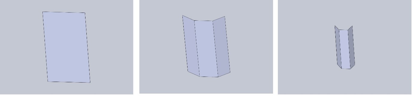
Figure 1 Sheet metal bent to form a gutter

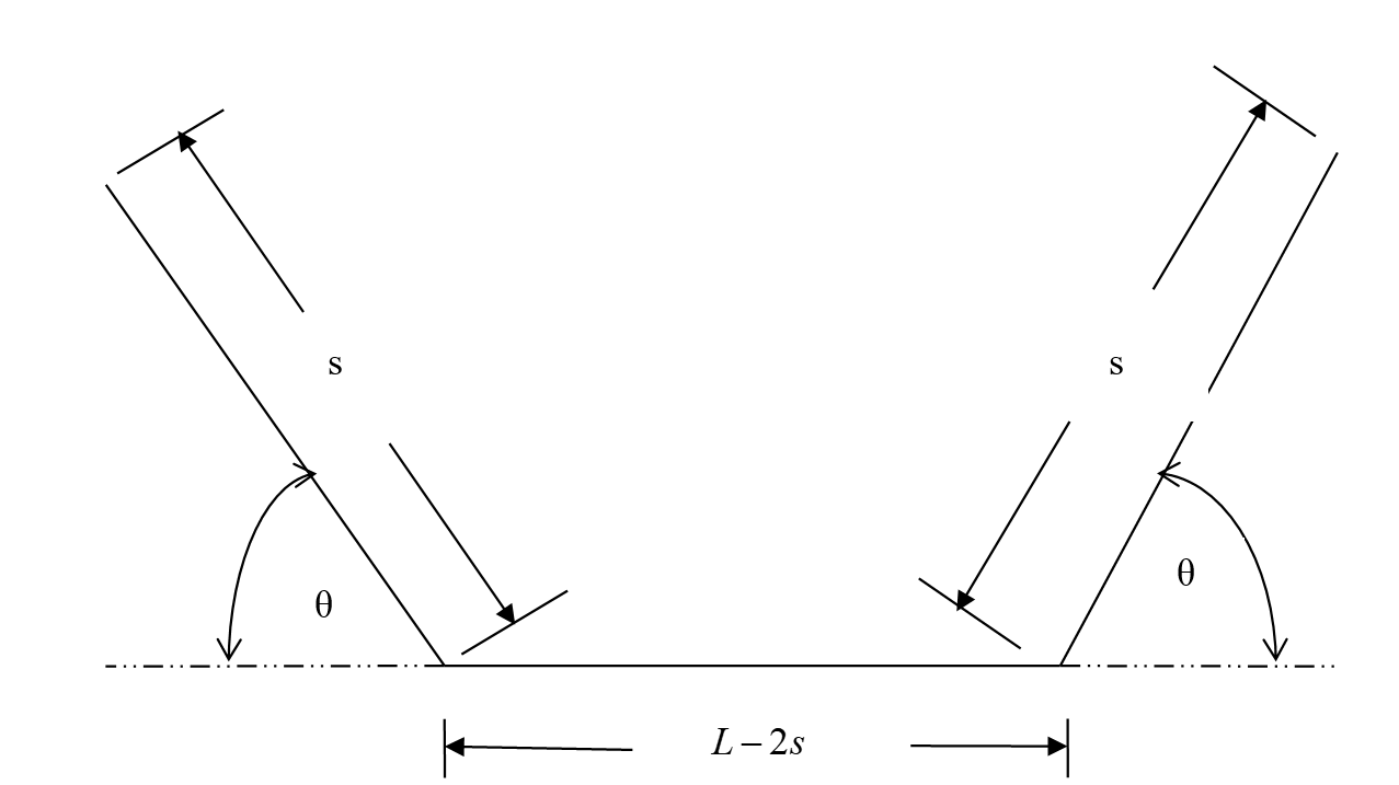
Figure 2: Labeling the parameters and points of the gutter

Solution

One needs to maximize the cross-sectional area of the gutter. The cross-sectional area $G$ of the gutter is given by

$$\begin{split} G &= \text{Area of trapezoid}\ \text{ABCD}\\ &= \frac{1}{2}(\text{AB} + \text{CD})(\text{FC})\;\;\;\;\;\;\; (E2.1)\end{split}$$

where

$$\text{AB}\ = \ L - 2\ s\;\;\;\;\;\;\; (E2.2)$$

$$\begin{split} CD &= AB + EA + BF\\ &= (L - 2s) + s\cos(\theta) + s\cos(\theta)\\ &= (L - 2s)\ + \ 2s\cos(\theta)\;\;\;\;\;\;\; (E2.3) \end{split}$$

$$\begin{split} FC &= BC \sin(\theta)\\ &= s\sin(\theta)\;\;\;\;\;\;\; (E2.4) \end{split}$$

hence

$$G = \frac{1}{2}(AB\ + CD) (DE)$$

$$\begin{split} G(s,\theta) &= \frac{1}{2}\left\lbrack (L - 2s) + (L - 2s) + 2s\cos(\theta) \right\rbrack s \sin(\theta)\\ &= \left\lbrack L - 2s + s\cos(\theta) \right\rbrack\ s\sin(\theta)\;\;\;\;\;\;\; (E2.5) \end{split}$$

For example, for $\theta = 0{^\circ}$, the cross-sectional area of the gutter becomes

$$G = 0$$

as it represents a flat sheet, for $\theta = 180{^\circ}$, the cross-sectional area of the gutter becomes

$$G = 0$$

as it represents an overlapped sheet, and for $\theta = 90{^\circ}$, it represents a rectangular cross-sectional area with

$$G = (L - 2s) s$$

For the given $L = 0.21\ \text{m,}$

$$G(s,\theta) = (0.21 - 2s + s\cos\theta)s\sin\theta$$

Then

$$\frac{\partial G}{\partial s} = - s^{2}\sin^{2}\theta + (0.21 - 2s + s\cos\theta)s\cos\theta$$

$$\frac{\partial G}{\partial\theta} = ( - 2 + \cos\theta)s\sin\theta + (0.21 + 2s + s\cos\theta)\sin\theta$$

By solving the equations

$$f_{1}(s,\theta) = - s\sin^{2}\theta + (0.21 - 2s + s\cos\theta)s\cos\theta = 0$$

$$f_{2}(s,\theta) = ( - 2 + \cos\theta)s\sin\theta + (0.21 - 2s + s\cos\theta)\sin\theta = 0$$

we can find the local minimas and maximas of $G(s,\theta)$. One of the local maximas may also be the absolute maximum. The values of $s$ and $\theta$ that correspond to the maximum of $G(s,\theta)$ are what we are looking for. Can you solve the equations to find the corresponding values of $s$ and $\theta$ for maximum value of $G$? Intuitively, what do you think would be these values of $s$ and $\theta$?

  

Appendix A: General matrix form of solving simultaneous nonlinear equations.

The general system of equations is given by

$$\begin{split} &f_{1}(x_{1},x_{2},...,x_{n}) = 0\\ &f_{2}(x_{1},x_{2},...,x_{n}) = 0\\ &\text{...}\\ &\text{...}\\ &\text{...}\\ &f_n(x_1,x_2,...,x_n) = 0\;\;\;\;\;\;\; (A.1)\end{split}$$

We can rewrite in a form as

$$F(\overset{\land}{x}) = \widehat{0}\;\;\;\;\;\;\; (A.2)$$

where

$$F(\overset{\land}{x}) = \begin{bmatrix} f_{1}(\overset{\land}{x}) \\ f_{2}(\overset{\land}{x}) \\ . \\ . \\ f_{n}(\overset{\land}{x}) \\ \end{bmatrix}\;\;\;\;\;\;\;(A.3)$$

$$\overset{\land}{0} = \begin{bmatrix} 0 \\ 0 \\ . \\ . \\ 0 \\ \end{bmatrix}\;\;\;\;\;\;\; (A.4)$$

$$\overset{\land}{x} = \begin{bmatrix} x_{1} \\ x_{2} \\ . \\ . \\ x_{n} \\ \end{bmatrix}^{T}\;\;\;\;\;\;\; (A.5)$$

The Jacobian of the system of equations by using Newton-Raphson method then is

$$J(x_{1},x_{2},...,x_{n}) = \begin{bmatrix} &\displaystyle\frac{\partial f_{1}}{\partial x_{1}}\ldots\frac{\partial f_{1}}{\partial x_{n}} \\ &.\ldots. \\ &.\ldots. \\ &.\ldots. \\ &\displaystyle\frac{\partial f_{n}}{\partial x_{1}}\ldots\frac{\partial f_{n}}{\partial x_{n}} \\ \end{bmatrix}\;\;\;\;\;\;\; (A.6)$$

Using the Jacobian for the Newton-Raphson method guess

$$\lbrack J\rbrack\Delta\overset{\land}{x} = - F(\overset{\land}{x})\;\;\;\;\;\;\; (A.7)$$

where

$$\Delta\overset{\land}{x} = {\overset{\land}{x}}_{\text{new}} - {\overset{\land}{x}}_{\text{old}}\;\;\;\;\;\;\; (A.8)$$

Hence

$$\Delta\overset{\land}{x} = - \lbrack J\rbrack^{- 1}F(\overset{\land}{x})$$

$${\overset{\land}{x}}_{\text{new}} - {\overset{\land}{x}}_{\text{old}} = - \lbrack J\rbrack^{- 1}F(\overset{\land}{x})$$

$${\overset{\land}{x}}_{\text{new}} = {\overset{\land}{x}}_{\text{old}} - \lbrack J\rbrack^{- 1}F(\overset{\land}{x})\;\;\;\;\;\;\; (A.10)$$

Evaluating the inverse of $\lbrack J\rbrack$ in Equation (A.10) is computationally more intensive than solving Equation (A.7) for $\Delta\overset{\land}{x}$and calculating ${\overset{\land}{x}}_{\text{new}}$ as

$${\overset{\land}{x}}_{\text{new}} = {\overset{\land}{x}}_{\text{old}} + \Delta\overset{\land}{x}\;\;\;\;\;\;\; (A.11)$$

Problem Set

(1).  Solve the following set of nonlinear equations using Newton-Raphson method.

$${xy = 2}$$

$${x^{2} + y = 5}$$ Start with an initial guess of $(3,4)$.

(2).  Write the drawbacks of Newton-Raphson method and how you would address them.

(3).  The following simultaneous nonlinear equations are found while modeling two continuous non-alcoholic stirred tank reactions

$${f_{1} = (1 - R)\left\lbrack \frac{D}{10(1 + \beta_{1})} - \varphi_{1} \right\rbrack\exp\left( \frac{10\varphi_{1}}{1 + 10\varphi_{1}/\gamma} \right) - \varphi_{1}}$$ $${f_{2} = \varphi_{1} - (1 + \beta_{2})\varphi_{2} + (1 - R) \times \left\lbrack \frac{D}{10} - \beta_{1}\varphi_{1} - (1 + \beta_{2})\varphi_{2} \right\rbrack\exp\left( \frac{10\varphi_{2}}{1 + 10\varphi_{2}/\gamma} \right)}$$

Given $\gamma = 1000,\ D = 22,\ \beta_{1} = 2,\ \beta_{2} = 2,\ R = 0.935$, find a suitable solution for $(\varphi_{1},\varphi_{2})$, given that $\varphi_{i} \in \left\lbrack 0,1 \right\rbrack,i = 1,2$

Source: Michael J. Hirsch, Panos M. Pardalos, Mauricio G.C Resende, Solving systems of nonlinear equations with continuous GRASP, Nonlinear Analysis: Real World Applications, Volume 10, Issue 4, August 2009, Pages 2000-2006, ISSN 1468-1218, http://dx.doi.org/10.1016/j.nonrwa.2008.03.006

(4).  The Lorenz equations are given by

$$\frac{dx}{dt} = \sigma(y - x)$$

$$\frac{{dy}}{{dt}} = x(p - z) - y$$

$$\frac{dz}{dt} = xy - \beta{z}$$

Assuming $\sigma = 3,\ p = 26,\ \beta = 1$, the steady state equations are written as

$${0 = 3(y - x)}$$ $${0 = x(26 - z) - y}$$ $${0 = xy - z}$$

Write the Jacobian for the above system of equations.

(5).  Use MATLAB or equivalent program to find the solution to the problem stated in Example 2.