Chapter 08.00: Physical Problem for Ordinary Differential Equations
Summary
To find the temperature of a heated ball as a function of time, a first-order ordinary differential equation must be solved.
Modeling
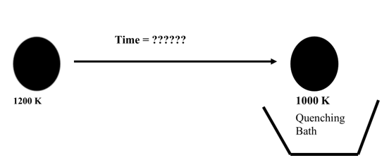
You are working for a ball bearing company - Ralph’s Bearings. For a long lasting life of some spherical bearings made in this company, after heating them to a high temperature of \(1000\ \text{K}\), they need to be quenched for \(30\) seconds in water that is maintained at a room temperature of \(300\ \text{K}\). However, it takes time to take the ball from the furnace to the quenching bath, and its temperature falls. The temperature of the furnace is \(1200\ \text{K}\), and it takes \(10\) seconds to take the ball to the quenching bath. Does the ball need to be in the air for less or more than \(10\) seconds to get to a temperature of \(1000\ \text{K}\)?
Mathematical model
To keep the mathematical simple, one can assume the spherical bearing to be a lumped mass system. What does a lumped system mean? It implies that the internal conduction in the sphere is large enough that the temperature throughout the ball is uniform. This assumption allows us to assume that the temperature is only a function of time and not of the location in the spherical ball. This dependence of temperature only on time for a lumped system means that if a differential equation governs this physical problem, it would be an ordinary differential equation. For a nonlumped system, a partial differential equation would govern. In your heat transfer course, you will learn when a system can be considered lumped or nonlumped. In simplistic terms, this distinction is based on the material, geometry, and heat exchange factors of the ball with its surroundings.
Now assuming a lumped-mass system, let us develop the mathematical model for the above problem. When the ball is taken out of the furnace at the initial temperature of \(\theta_{0}\) and is cooled by radiation to its surroundings at the temperature of \(\theta_{a}\), the rate at which heat is lost to radiation is
\[\text{Rate of heat lost due to radiation} = A \epsilon \sigma\left( \theta^{4} - {\theta_{a}}^{4} \right)\;\;\;\;\;\;\;\;\;\;\;\; (1)\]
where
\[A = \text{surface area of the ball,}\ \text{m}^{2}\]
\[\epsilon = \text{emittance}\]
\[\sigma = \text{Stefan-Boltzmann constant,}\ 5.67 \times 10^{- 8}\ \frac{\text{J}}{\text{s}\cdot \text{m}^{2}\cdot \text{K}^{4}}\]
\[\theta = \text{temperature of the ball at a given time,}\ \text{K}\]
In the above equation for radiation heat loss, emittance \(\epsilon\) is defined as the total radiation emitted divided by total radiation that would be emitted by a blackbody at the same temperature. The emittance is always between \(0\) and \(1\). A black body is a body that emits and absorbs at any temperature the maximum possible amount of radiation at any given wavelength.
Stefan-Botzmann constant, \(\sigma\) was discovered by two Austrian scientists – J. Stefan and L. Boltzmann. Stefan found it experimentally in 1879, and Boltzmann derived it theoretically in 1884.
The energy stored in the mass is given by
\[\text{Energy stored by mass} = mC\theta\;\;\;\;\;\;\;\;\;\;\;\; (2)\]
where
\[m = \text{mass of the ball,}\ \text{kg}\]
\[C = \text{specific heat of the ball,}\ \text{J}/\left( \text{kg} - \text{K} \right)\]
From an energy balance,
\[\begin{split} &\text{Rate at which heat is gained} - \text{Rate at which heat is lost}\\ &=\text{Rate at which heat is stored} \end{split}\]
gives
\[- A \epsilon \sigma\left( \theta^{4} - \theta_{a}^{4} \right) = mC\frac{{d\theta}}{{dt}}\;\;\;\;\;\;\;\;\;\;\;\; (3)\]
Given the
\[\text{Radius of the ball,}\ r = 2.0\ \text{cm}\]
\[\text{Density of the ball,}\ \rho = 7800\ \text{kg/m}^{3}\]
\[\text{Specific heat,}\ C = 420\ \text{J}/(\text{kg}\cdot \text{K})\]
\[\text{Emittance,}\ \in = 0.85\]
\[\text{Stefan-Boltzmann Constant,}\ \sigma = 5.67 \times 10^{-8}\ \frac{\text{J}}{\text{s}\cdot \text{m}^{2}\cdot \text{K}^{4}}\]
\[\text{Initial temperature of the ball,}\ \theta\left( 0 \right) = 1200\ \text{K},\]
\[\text{Ambient temperature,}\ \theta_{a} = 300\ \text{K},\]
we have
Surface area of the ball
\[\begin{split} A &= 4\pi r^{2}\\ &= 4\pi\left( 0.02 \right)^{2}\\ &= 5.02654 \times 10^{- 3}\text{m}^{2} \end{split}\]
Mass of the ball
\[\begin{split} M &= pV\\ &= \rho\left\lbrack \frac{4}{3}\pi r^{3} \right\rbrack\\ &= 7800 \times \left( \frac{4}{3} \right)\pi(0.02)^{3}\\ &= 0.261380\ \text{kg} \end{split}\]
Hence
\[- A \epsilon \sigma(\theta^{4} - {\theta_{a}}^{4}) = mC\frac{{d\theta}}{{dt}}\;\;\;\;\;\;\;\;\;\;\;\; (3 - repeated)\]
reduces to
\[- (5.02654 \times 10^{- 3})(0.85)(5.67 \times 10^{- 8})(\theta^{4} - 300^{4}) = (0.261380)(420)\frac{{d\theta}}{{dt}}\]
\[\frac{{d\theta}}{{dt}} = - 2.20673 \times {1}{0}^{- 12}\ (\theta^{4} - 81 \times 10^{8})\;\;\;\;\;\;\;\;\;\;\;\; (4)\]
An improved mathematical model
The heat from the ball can also be lost due to convection. The rate of heat lost due to convection is
\[\text{Rate of heat lost due to convection} = hA\left( \theta - \theta_{a} \right),\;\;\;\;\;\;\;\;\;\;\;\; (5)\]
where
\[h = \text{the convective cooling coefficient},\ \left\lbrack \text{W}/\left( \text{m}^{2} - \text{K} \right) \right\rbrack.\]
Hence the heat is lost is due to convection as well as radiation and is given by
\[\text{Rate of heat lost due to convection and radiation} = A \in \sigma\left( \theta^{4} - \theta_{a}^{4} \right) + hA\left( \theta - \theta_{a} \right)\]
\[\text{Energy stored by mass} = mC\theta\;\;\;\;\;\;\;\;\;\;\;\; (6)\]
From an energy balance,
\[\begin{split} &\text{Rate at which heat is gained} -\text{Rate at which heat is lost}\\ &=\text{Rate at which heat is stored} \end{split}\]
gives
\[- A \epsilon \sigma\left( \theta^{4} - \theta_{a}^{4} \right) - hA\left( \theta - \theta_{a} \right) = mC\frac{{d\theta}}{{dt}}\;\;\;\;\;\;\;\;\;\;\;\; (7)\]
Given \(h = 350\frac{J}{s - m^{2} - K}\) and considering both convection and radiation, and substituting the values of the constants given before
\[- (5.02654 \times 10^{- 3})(0.85)(5.67 \times 10^{- 8})(\theta^{4} - 300^{4})\]
\[- (350)(5.02654 \times 10^{- 3})(\theta - 300) = (0.261380)(420)\frac{{d\theta}}{{dt}}\]
\[\frac{{d\theta}}{{dt}} = - 2.20673 \times 10^{- 13}(\theta^{4} - 81 \times 10^{8}) - 1.60256 \times 10^{- 2}(\theta - 300)\;\;\;\;\;\;\;\;\;\;\;\; (8)\]
The solution to the above ordinary differential equation with the initial condition of \(\theta\left( 0 \right) = 1200\ \text{K}\) would give us the temperature of the ball as a function of time. We can then find at what time the ball temperature drops to \(1000\ \text{K}\).
Questions
(1) Note that the ordinary differential equation given by Equation (8) is non-linear. Is there is an exact solution to the problem?
(2) You are asked to solve the inverse problem, that is, when will the dependent variable temperature equal to \(1000\ \text{K}\). How would you solve the inverse problem using different numerical methods such as Euler’s and Runge-Kutta’s methods?
(3) Can you find if convection or radiation can be neglected? How would you quantify the effect of neglecting one or the other?
(4) Find the following at \(t = 5\text{ s}\)
Rate of change of temperature,
Rate at which heat is lost due to convection,
Rate at which heat is lost due to radiation,
Rate at which heat is stored in the ball.
Summary
Sodium chloride waste control while making soap requires solution of an ordinary differential equation
Modeling
Soap is prepared through a reaction known as saponification. In saponification, tallow (fats from animals such as cattle) or vegetable fat (e.g. coconut) is reacted with potassium or sodium hydroxide to produce glycerol and fatty acid salt known as “soap”. The soap is separated from the glycerol through precipitation by the addition of sodium chloride. Water layer on top of the mixture that contains dissolved sodium chloride is drawn-off the mixture as a waste. This method of soap making is still being practiced in many villages in the developing countries where the price of mass produced soap maybe too expensive for the average villager.
Two chemical engineering students used knowledge of saponification acquired in their organic chemistry class to organize and produce “home made” soap. The local ordinance requires that the minimum concentration level for sodium chloride waste in any liquid that is discharged into the environment must not exceed \(11.00\) g/L. Sodium chloride laden liquid water is the major waste of the process. The company has only one 15-liter tank for waste storage. On filling the waste tank, the tank contained \(15\) liters of water and \(750\) grams of sodium chloride. To continue production and meet local ordinance, it is desired to pump in fresh water into the tank at the rate of \(2.0\) liters per minute while waste salt water containing \(25\) grams of salt per liter is added at the rate of \(1.5\) liters per minute. To keep the solution level at \(15\) liters, \(3.5\) liters per minute of the waste is discharged. A sketch Figure 1 of the flows is given below where \(A\) represents the waste stream from the process, \(B\) is the fresh water stream and \(C\) is the discharge stream to the environment. Here, it is assumed that as the two streams, \(A\) and \(B\) enter into the tank, instantaneously the chloride concentration in the tank changes to the exit concentration,\({X}_{1}\).
The material (sodium chloride) balance on the tank system can be written as
\[\text{Accumulation} = \text{input} - \text{output} + \text{removal by reaction} \ \ \ (1)\]
Noting that no chemical reaction occurs in the storage tank (i.e. the third term on the right hand side of (1) is zero), the above equation can be written as
\[\frac{dx_{1}}{{dt}} = (25{g/L})(1.5{L/min}) + (0{g/L})(2{L/min}) - (x_{1}{g/L})(3.5{L/min}) + 0\ \ \ (2)\]
Simplifying Equation (2), we obtain
\[\frac{dx_{1}}{{dt}} + 3.5x_{1} = 37.5\ \ \ (3)\]
For the initial conditions of the ordinary differential equations in Equation (3), recall that at \(t = 0\), the salt concentration in the tank was given as 750 g/15L (50g/L) , that is,
\[t = 0,x_{1}(0) = \frac{750}{15} = 50{g/L}\ \ \ (4)\]
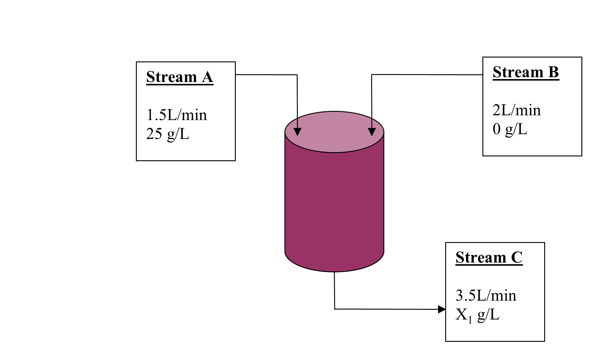
Figure 1 Sketch of flow for a saponification process.
Question
(1) Using Equations (3) and (4), numerically determine how the concentration of salt being discharged changes with time.
(2) Plot the solution obtained.
(3) How long did it take to achieve the minimum required local ordinance? At steady state, what is the concentration of salt being discharged from this local soap factory?
Summary
A physical problem of finding how much time it would take a lake to have safe levels of pollutant. To find the time, the problem is modeled as an ordinary differential equation.
Modeling
Pollution in lakes can be a serious issue as they are used for recreation use. Pollution resulting from sewage, runoff from suburban yards that is loaded with fertilizers and pesticides to keep the homeowner’s associations off your back can be a safety hazard for people. One is generally interested in knowing that if the concentration of a particular pollutant is above acceptable levels, how long will it take for the pollution level to decrease to an acceptable level.
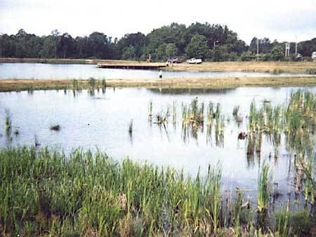
Figure 1 Pollutant in a lake
\[\text{Mass of pollutant} = \text{Mass of pollutant entering} - \text{Mass of pollutant leaving}\]
which also gives
\[\begin{split} &\text{Rate of change of mass of pollutant} = \text{Rate of change of mass of pollutant entering}\ - \\ & \text{Rate of change of mass of pollutant leaving.}\end{split}\]
If the concentration of pollutant is given by
\[C\left( t \right) = \frac{M\left( t \right)}{V}\]
where
\[M\left( t \right) =\text{mass of pollutant at time}\ t\]
\[V =\text{Volume of lake.}\]
Rate of change of mass of pollutant entering is \(QC_{o}\), where \(Q\) is the flow rate of the water into the lake, and the rate of change of mass of pollutant leaving the lake is \(\displaystyle \frac{{QM}\left( t \right)}{V}\).
The above assumes that the flow rate of water going in and out of lake is the same. We also assuming that the pollutant is uniformly distributed in the lake. Also, no reaction is assumed. This gives
\[\frac{{dM}\left( t \right)}{{dt}} = QC_{o} - \frac{\dot{Q}M\left( t \right)}{V}\]
Now
\[M\left( t \right) = VC_{o}\left( t \right)\]
giving
\[V\frac{{dC}}{{dt}} = \dot{Q}C_{o} - \dot{Q}C\]
\[V\frac{{dC}}{{dt}} + \dot{Q}C = \dot{Q}C_{o}\]
Assume a weekly flow rate of fresh water as \(1.5 \times 10^{6}m^{3}\). \(C_{o} = 0\) as we are assuming only fresh water coming in. The volume of the lake is \(25 \times 10^{6}m^{3}\). If the initial concentration of the pollutant is \(10^{7}{parts}/m^{3}\), and the acceptable level is \(5 \times 10^{6}{parts}/m^{3}\), how much time would it take for the pollutant to reach acceptable levels.
\[25 \times 10^{6}\frac{{dC}}{{dt}} + 1.5 \times 10^{6}C = 0\]
\[\frac{{dC}}{{dt}} + 0.06C = 0,C\left( 0 \right) = 10^{7}\]
Summary
Transient analysis of resistor-capacitor requires solution of ordinary differential equations.
Modeling
Resistors and capacitors are fundamental elements of any circuit. Even the behavior of semiconductor devices in your computer can be modeled employing these basis elements (along with some others). A transistor is comprised of junctions of different kinds of materials, giving rise to interesting electrical properties. The electrical properties at these semiconductor junctions can be characterized using resistors (R) and capacitors (C), giving rise to the name “RC-model”. In this module we will consider the electrical behavior of the simplest configuration of the RC elements and see how it can characterized using ordinary differential elements.
Two quantities that are important in electrical circuits are voltage (denoted here by V) and current (denoted here by I). The current through a resistor has a linear relationship with voltage and is defined by \(V = IR\), where R, is constant used to quantify the resistor. This is called the Ohms law and you should have seen it one of your physics classes. A capacitor is a bit stranger element for which the rate of change of voltage across it is proportional to the current. Or in other words: \(C\frac{{dV}}{{dt}} = I\), where C is called the capacitance. Voltage changes slowly across high capacitance. These elements are represented by diagrams as shown below.
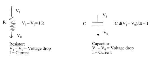
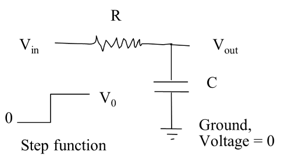
Figure 1. A simple RC circuit. As the input voltage is switched on at t=0, what happens to the output voltage.
Consider the simple combination of resistor and capacitor, as shown above. This kind of configuration is not rare and occurs in all power supplies to your computer. There are other components in addition to this, but this is one of the basic arrangements. The voltage at one end of the resistor is denoted by Vin and the voltage at the other end is denoted by Vout. The latter end is also connected to the capacitor, whose other end of which is connected to ground, which can be taken to be at zero voltage. The question we ask is what happens to the output voltage Vout when the input voltage Vin is switched on suddenly?
The voltage and current relationship across the resistor and the capacitor can be expressed, respectively as
\[V_{{in}} - V_{{out}} = IR \ \text{and}\]
\[C\frac{dV_{{out}}}{{dt}} = I\]
where I is the current through the circuit. Eliminating this quantity from the above two equations, we have
\[V_{{in}} - V_{{out}} = RC\frac{dV_{{out}}}{{dt}}\]
For any input voltage profile we can solve this equation to arrive at the output voltage profile.
Worked Out Example
The sudden change in the input voltage can be modeled using the following function
\[V_{{in}} = \left\{ \begin{matrix} \begin{matrix} V_{0} & \ & \forall t \geq 0 \\ \end{matrix} \\ \begin{matrix} 0 & \ & \forall t < 0 \\ \end{matrix} \\ \end{matrix} \right.\ \]
This is also called a “step” function. For this input the differential equation modeling the output voltage for \(t>0\) is given by
\[{RC}\frac{dV_{{out}}}{{dt}} = V_{0} - V_{{out}}\]
The solution of this equation we need some boundary conditions. We know the voltage at \(t = 0\) is zero, i.e. \(V_{{out}}(0) = 0\), and the voltage after a long time should be equal to the new input voltage, i.e \(V_{{out}}(\infty) = V_{0}\). Using boundary conditions, in along with general solution form: \(V_{{out}}(t) = c_{o}\exp(at) + c_{1}\exp( - at) + c_{2}\), we can arrive at the following solution for the output voltage
\[V_{{out}}(t) = V_{o}(1 - \exp( - \frac{t}{{RC}}))\]
In the Figure 2 we see the plot of the transient output voltage for various values of the product RC. The output starts at zero and gradually converges to V0 = 1. The rate of convergence is dependent on the product RC.
Questions
(1) If the for \(V_{{in}} = x_{1}(t)\), the output voltage is given by the function \(y_{1}(t)\), and for \(V_{{in}} = x_{2}(t)\), the output voltage is given by the function \(y_{2}(t)\), show that the output for the input \(V_{{in}} = x_{1}(t) + x_{2}(t)\), is given by \(y_{1}(t) + y_{2}(t)\).
(2) If the for \(V_{{in}} = x_{1}(t)\), the output voltage is given by the function \(y_{1}(t)\), show that the output for the input \(V_{{in}} = ax_{1}(t)\), is given by \(ay_{1}(t)\).
(3) Consider a pulse shaped input that is defined by:
\[V_{{in}}(t) = \left\{ \begin{matrix} \begin{matrix} 0 & \ & \forall t < 0 \\ \end{matrix} \\ \begin{matrix} V_{0} & \ & 0 \leq t \leq T \\ \end{matrix} \\ \begin{matrix} 0 & \ & t > T \\ \end{matrix} \\ \end{matrix} \right.\]
What is the form of the output?
Hint: Express this input of in the form \(x_{1}(t) - x_{2}(t)\) and then use the properties you have derived so far to arrive at the solution.
(4) What can you say about the output as the ratio \(\frac{T}{{RC}}\) is varied?
(5) What can say about the behavior of this circuit when there is a voltage “spike” at the input?
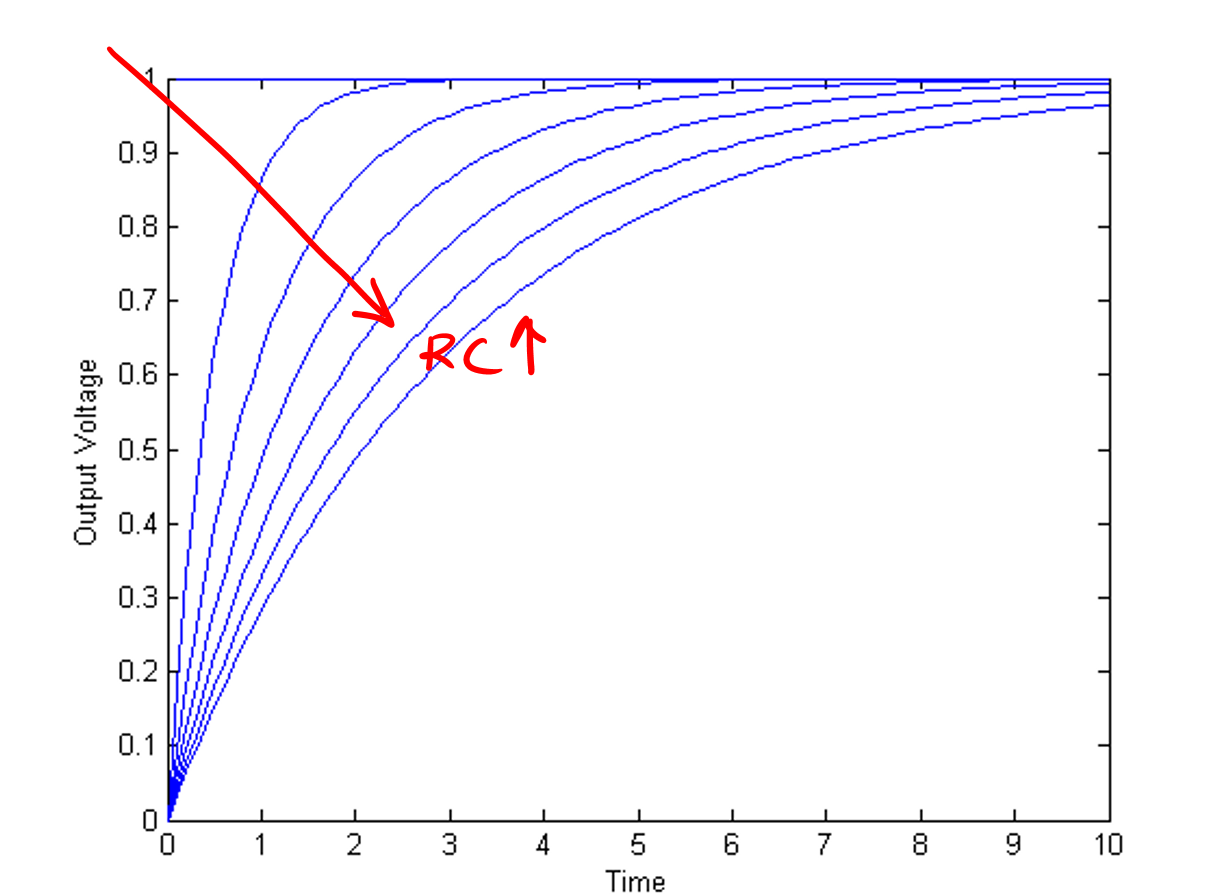
Figure 2. Output voltage, Vout(t), for various values of the product RC.
Summary
A rectifier-based power supply requires a capacitor to store power temporarily when the rectified waveform from the AC source drops below the target voltage. To size this capacitor properly, a first-order ordinary differential equation must be solved.
Modeling
Small non-switching power supplies such as AC power bricks are typically built around a small transformer, rectifier, and voltage regulator as shown in Figure 1.
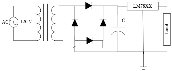
Figure 1. Full-Wave Rectified DC Power Supply
The transformer is used to reduce the AC voltage levels to a more reasonable range (e.g. 12 VAC or 18 VAC) and the bridge rectifier will take the negative half cycle of the AC waveform and convert it to a positive half cycle. A typical full-wave rectified waveform is shown in Figure 2. This waveform was generated assuming an ideal diode operating under no-load conditions and can be modeled with the following equation:
\[V_{\text{full}} = \max\left( \left| 18 \times \cos\left( t \right) - 1.4 \right|,0 \right)\]
For a half-wave rectified system built using only a single diode, the equation would become:
\[V_{h\text{alf}} = \max\left( 18 \times \cos\left( t \right) - 0.7,0 \right)\]
and the waveform would look similar to Figure 2 except every other hump would be replaced with 0.
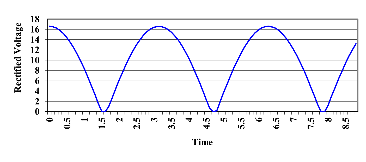
Figure 2 Full-Wave Rectified AC Signal.
This is clearly not suitable as a DC power source since the load is looking for a constant DC value. This is where the capacitor, C, and the LM78XX voltage regulator of Figure 1 become important. A typical voltage regulator requires that the voltage on the input pin maintain a certain margin above the regulated output voltage. This is typically in the range of 2.5 to 3 V and for the LM7805, which provides 5 VDC, it is 2.5 V [1]. This means that the minimum voltage at the input pin of the LM7805 must not drop below 7.5 V. Clearly, the waveform in Figure 2 does that regularly.
The task of the capacitor, C, in the power supply is to store up charge when the rectifier provides voltage in excess of the required minimum and then support the voltage when the regulated voltage is below the minimum by providing stored charge to the voltage regulator. Thus, the circuit has two distinct phases of operation.
Phase 1
When the rectified voltage is above the voltage across the capacitor \(V_{c}\), then the rectifier provides current to the capacitor and the voltage regulator, and the capacitor charges. The ideal model of a diode will not be adequate here since we need to know how much current the diode can supply. A better model of the diode can be found from its VI characteristic such as the one shown in Figure 3. A model for this will be developed shortly.
Phase 2
When the rectified voltage drops below \(V_{c}\) current ceases to flow between the rectifier diodes and the capacitor. The capacitor then becomes the sole source of current to the voltage regulator by bleeding off its charge. This has the additional effect of continually reducing the voltage across the capacitor. As long as it does not fall below the required threshold, the regulator can successfully do its job.
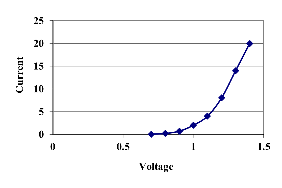
Figure 3 VI Characteristic of a 1N4001 Diode [2].
Diode Model
The diode of Figure 3 must be modeled to account properly for the current it can supply during the Phase 1 charging phase of the capacitor. It is reasonable to model a diode under these conditions as a voltage drop and a series resistance. This essentially treats the Figure 3 curve as piece-wise linear model and it can only be applied when the diode is on (that is, it does not properly model an under-biased or reverse-biased diode) [3, pp. 67-74]. This model is shown in Figure 4 and for the 1N4001 of Figure 3 suitable values are \(V_{d} = 1.0\ V\) and \(R_{d} = 0.02\ \Omega\). Other diodes will have similar numbers.
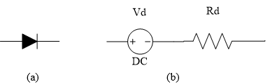
Figure 4 (a) Ideal Diode and (b) Piece-wise Forward Bias Model.
Load Model
The final piece to the picture is how to model the load represented by the voltage regulator. Rather than get into the details of the internal structure of the voltage regulator it is sufficient to model the worst-case scenario when choosing the appropriate capacitor. This is represented by the peak continuous current that the power-supply is expected to provide. For this problem, it will be assumed to be 100 mA.
Circuit Models
With the Phase 1 charging, and Phase 2 discharging, circuit models of the power supply circuit can now be built. They are shown in Figure 5. In both cases, the circuit must provide 100 mA to the load. It will be additionally assumed that a transformer will be chosen that provides sufficient AC power at 18 VAC running at 60 Hz.
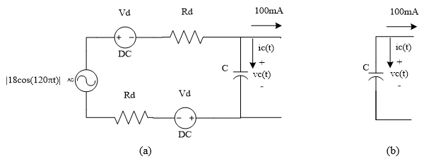
Figure 5 (a)Phase 1 (Charging) and (b) Phase 2 (Discharging) Circuit Models
Analysis
The analysis of these two circuits is rather straight-forward once the VI characteristic of the capacitor is substituted. In the time-domain, this is represented by the differential equation
\[i_{c}\left( t \right) = C\frac{dv_{c}\left( t \right)}{{dt}}\ \text{subject to initial conditions on}\ v_{c}.\]
During the charging of Phase 1, the operative circuit equation is found by writing a Kirchoff’s Current Law equation for the node at the top of the capacitor. Doing this yields
\[C\frac{dv_{c}\left( t \right)}{{dt}} + 100mA = \frac{\left| 18\cos\left( 120\pi t \right) \right| - 2V_{d} - v_{c}\left( t \right)}{2R_{d}},\]
when
\[v_{c}\left( t \right) \leq \left| 18\cos\left( 120\pi t \right) \right| - 2V_{d}.\]
During the discharging of Phase 2, the circuit is a bit simpler and the equation is
\[C\frac{dv_{c}\left( t \right)}{{dt}} + 100mA = 0,\]
when
\[v_{c}\left( t \right)\rangle\left| 18\cos\left( 120\pi t \right) \right| - 2V_{d}.\]
These are essentially the same differential equation it is just that the forcing function has two cases that must be monitored as the equation is solved. Substituting the previously derived values for \(V_{d}\) and \(R_{d}\) will yield the following equation in standard form.
\[\frac{dv_{c}\left( t \right)}{\text{dt}} = \frac{1}{C}\left\{ - 0.1 + \max\left( \frac{\left| 18\cos\left( 120\pi t \right) \right| - 2 - v_{c}\left( t \right)}{0.04},0 \right) \right\}.\]
Assuming that the capacitor is initially discharged (i.e.\(v_{c}\left( 0 + \right) = 0\)) it is simply a matter of trying various standard capacitors (e.g. \(100, 150, 220, 330, 470,\) and \(680 {\mu F}\) or other powers of \(10\) [4]) into the equation and simulating it for a few cycles of the AC source. Pick the smallest value where \(v_{c}\left( t \right)\) never drops below the required \(7.5\ V\).
Questions
(1) Most capacitors are marked with a tolerance of\(\pm 20\%\). How would your analysis handle the case that a \(100\ \mu F\)capacitor could be as high as \(120\ \mu F\) or as low as\(80\ \mu F\)?
(2) What effect would it have on the differential equation to use a more complex model for the diode?
(3) Is it necessary to have a more detailed model of the voltage regulator? Alternatively, is it suitable to model it simply as a maximum current sink?
(4) Modify the model to account for an AC brownout, that is, what would happen if the AC power source saw a temporary drop in voltage?
References
[1] LM340/LM78XX Data Sheet, National Semiconductor, http://www.national.com/ds/LM/LM340.pdf, accessed May 11, 2005.
[2] 1N4001 Data Sheet, Fairchild Semiconductor, http://www.fairchildsemi.com/ds/1N/1N4007.pdf, accessed May 12, 2005.
[3] Malvino, A., Electronic Principles, Sixth Edition, Glencoe McGraw-Hill, 1999.
[4] Standard Capacitor Values, RF Café, http://www.rfcafe.com/references/electrical/capacitor_values.htm, accessed May 12, 2005.
Summary
Many appliances used in our daily lives as well as numerous applications in industrial automation require controlling speed of a DC motor to function properly. Classical control theory requires solving differential equations to control these types of motors.
Modeling
In this example we will discuss the closed loop speed control of a DC motor. Figure 1 shows three different DC motors and Figure 2 depicts the inside of a DC motor. Universal Motors which are essentially DC motors are widely used in applications where the speed of a process needs to be controlled. Such applications are encountered frequently in our daily lives such as controlling the speed of fans or controlling the speed of hand-held tools such as drills, and in industrial automation applications such as controlling the speed of conveyor belts.
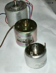
Figure 1 A variety of DC motors
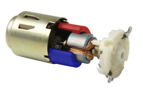
Figure 2 The inside of a DC motor
Before we can discuss the speed control of a DC motor, it is important to understand the physical time varying relationships that determine the operating characteristics of a DC motor.
Equation (1) below describes the linear relationship between the torque \(T\) and the current \(i_{a}\) applied to the motor. The slope of the line is the torque constant \(K_{t}\). Equation (2) describes the linear relationship between the back emf \(E_{B}\) and the armature speed \(w\). The slope of the line \(K_{B}\) is the voltage constant. Equation (3) describes the components of the armature voltage \(V\) as sum of the back emf and the voltage drop across armature resistance \(Ri_{a}\). Finally, Equation (4) describes the relationship between torque, acceleration and speed of the motor in a no-load system as the sum of the angular acceleration \(dw/dt\) multiplied by the inertia of the motor and the load, and the damping of the system \(f\) multiplied by the armature speed.
\[T(t) = K_{T}i_{a}(t)\ \ \ (1)\]
\[E_{B}(t) = K_{B}w(t)\ \ \ (2)\]
\[V(t) = Ri_{a}(t) + E_{B}(t)\ \ \ (3)\]
\[T(t) = I\frac{{dw}}{{dt}} + fw(t)\ \ \ (4)\]
The equation for the speed of the motor in relation to the voltage input can be derived from these relationships as follows. Substitute the value of back emf from Equation (2) into Equation (3) as:
\[V(t) = Ri_{a}(t) + K_{B}w(t)\ \ \ (5)\]
Equating Equations (1) and (4) and solving for ia results in
\[i_{a} = \frac{I\frac{{dw}}{{dt}} + fw(t)}{K_{T}}\ \ \ (6)\]
Finally substitute the value for ia from Equation (6) into Equation (5) as
\[K_{T}V(t) = RI\frac{{dw}}{{dt}} + (Rf + K_{T}K_{B})w(t)\ \ \ (7)\]
Equation (7) is a first order differential equation which describes the open-loop response of the motor to a voltage input where the output variable system (speed of the motor) is not considered in the control mechanism. In the next section we will consider the closed-loop control of the motor.
Closed loop control
Figure 3 illustrates the block diagram of a proportional control system used to control the speed of a DC motor where KP is the proportional gain. The “C” block is the summing point which generates an error term e equal to the difference between the desired speed set by the operator (\(w_{d}\)) and the actual speed of the motor. The “DC Motor” block transforms the amplified error input from the “Control Action” block to the output speed of the motor.
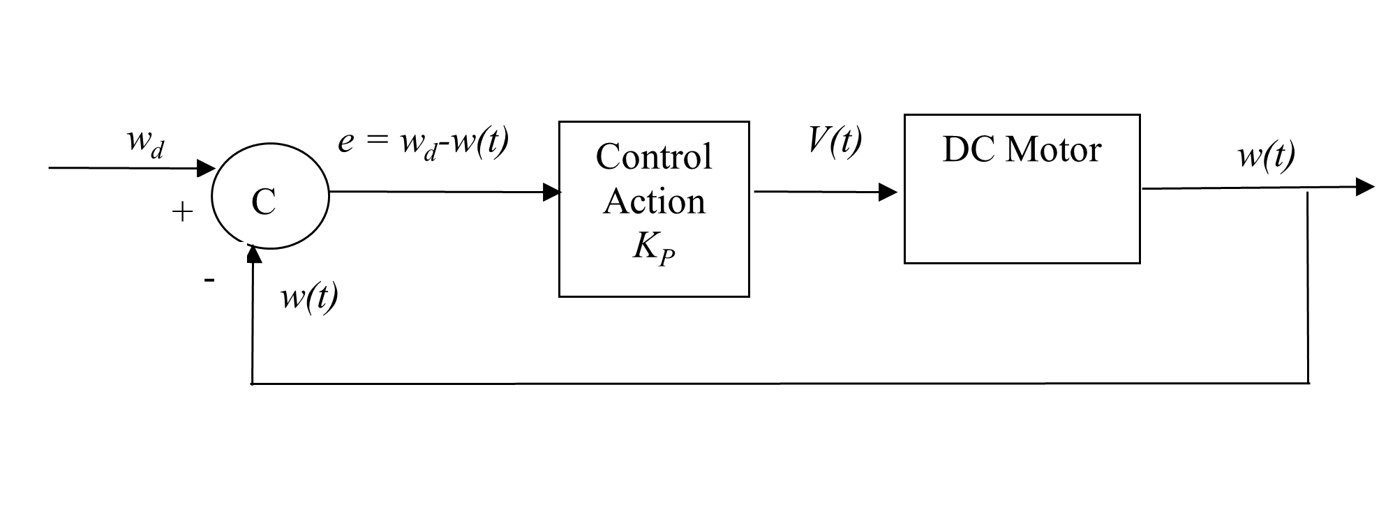
Figure 3 Block diagram of a DC motor control systems
Based on the control system block diagram
\[V(t) = K_{P}\lbrack w_{d} - w(t)\rbrack\ \ \ (8)\]
Substituting the value of \(V\left( t \right)\)from Equation (8) in to Equation (7) and rearranging terms results in the differential Equation (9) which describes the relationship of the actual speed of the motor to the desired speed.
\[K_{T}K_{P}w_{d} = RI\frac{{dw}}{{dt}} + \lbrack Rf + K_{T}(K_{B} + K_{P})\rbrack w(t)\ \ \ (9)\]
Example application
Consider a machine vision quality inspection system which inspects parts for defects shown in Figure 4. The parts are positioned in fixtures on a conveyor driven by a DC motor. The conveyor is required to ramp up to a certain speed within a specific time (before a part enters the field of view of the camera), maintain a constant speed while the part is under the camera and finally come to a stop once the inspection of the part is completed. Many such applications which utilize DC motors have requirements associated with the steady-state speed and/or a ramp up time for the motor to reach this speed.
Consider a DC motor which has the following specifications:
\[\text{Voltage constant,}\ K_{B}= 0.06 V.s/rad\]
\[\text{Torque constant,}\ K_{t}= 0.06 N.m/A\]
\[\text{Armature resistance,}\ R = 2 \Omega\]
\[\text{Moment of inertia,}\ I = 6 \times 10^{- 4}{N.m.}{s}^{2}{/rad}\]
The open loop response of the motor to a voltage input using Equation (7) and assuming a system without damping ((\(f\) = 0 N.m.s /rad)) is
\[V(t) = ({0.02})\ \frac{{dw}}{{dt}} + (0.06)w(t).\]
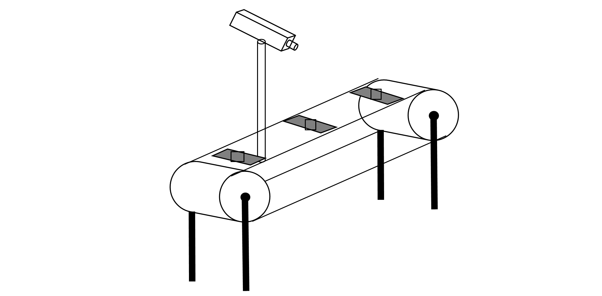
Figure 4 Machine vision system schematic
The speed of the motor \(w\left( t \right)\) can therefore be controlled by changing the magnitude of this input voltage (\(v\left( t \right)\)). Assuming the initial condition \(w\left( 0 \right) = 0\)and a specific input voltage, the above ordinary differential equation can be solved to determine the stead-state speed of the motor as well as the time it takes for the motor to ramp up to this speed. The information obtained from the solution is important in selection of the appropriate voltage input and/or motor for a particular application to assure that the motor response time and speed is sufficient for the task.
Similarly, the design of a closed loop controller to control the speed of the motor requires the solution to the ordinary differential Equation (9) to determine the user settings to obtain the necessary output from the motor. This application is posed as Exercise Problem 5 below.
Questions
For the DC motor in the Example Problem, answer the following questions:
(1) Draw the speed response graph \(w\left( t \right)\) vs \(t\) for a step input of 20 Volts without the damping of the system (\(f = 0\; N.m.s/rad\))
(2) Draw the speed response graph for a step input of 20 Volts considering the damping of the system where \(f = 1.0 \times 10^{- 4}{N.m.s/rad}\).
(3) What is the difference between the steady-state speed of the motor with and without damping?
(4) Consider a closed loop control system with gain \(K_{P} = 10\). What is the closed loop speed response graph of motor to a desired setting of 100 rad/s?
(5) The answer to Question #4 is less than 100 rad/s due to the steady state error present in first order systems. What should be the desired speed setting for the motor speed response to be 100 rad/s?
References
[1] Boucher, T.O., Computer Automation in Manufacturing: An Introduction, Chapman & Hall, London, 1996.
[2] Bateson, R.N., Introduction to Control System Technology, 6th Edition, Prentice Hall, New Jersey, 1999.
Summary
A physical problem of finding how much time it would take a trunnion to cool down in a refrigerated chamber is presented. To estimate this time, the problem would be modeled as an ordinary differential equation.
Modeling
To make the fulcrum (Figure 1) of a bascule bridge, a long hollow steel shaft called the trunnion is shrink fit into a steel hub. The resulting steel trunnion-hub assembly is then shrunk-fit into the girder of the bridge.
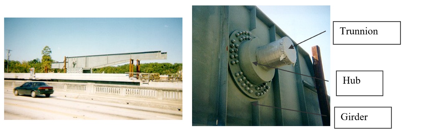
Figure 1 Trunnion-Hub-Girder (THG) assembly.
This assembly is done by first immersing the trunnion in a cold medium such as liquid nitrogen. After the trunnion reaches the steady-state temperature, that is, the temperature of the cold medium, the trunnion outer diameter contracts. The trunnion is taken out of the medium and slid though the hole of the hub (Figure 1).
When the trunnion heats up, it expands and creates an interference fit with the hub. Because of the large thermal shock that the trunnion undergoes, it is suggested that the trunnion be cooled in stages. First, put the trunnion in a refrigerated chamber, then dip it in a dry-ice/alcohol mixture and then immerse it in a bath of liquid nitrogen. However, this approach will take more time. One is mainly concerned about the cooling time in the refrigerated chamber. Assuming that the room temperature is \(27^{\circ} \text{C}\) and the refrigerated chamber is set is \(-33^{\circ} \text{C}\), how much time would it take for the trunnion to cool down to \(-33^{\circ} \text{C}\)?
Let us do a simplified problem of a solid trunnion and assume the trunnion can be treated as a lumped-mass system. What does a lumped system mean?
Let us develop the mathematical model for the above problem. When the trunnion is placed in the refrigerated chamber, the trunnion loses heat to its surroundings by convection.
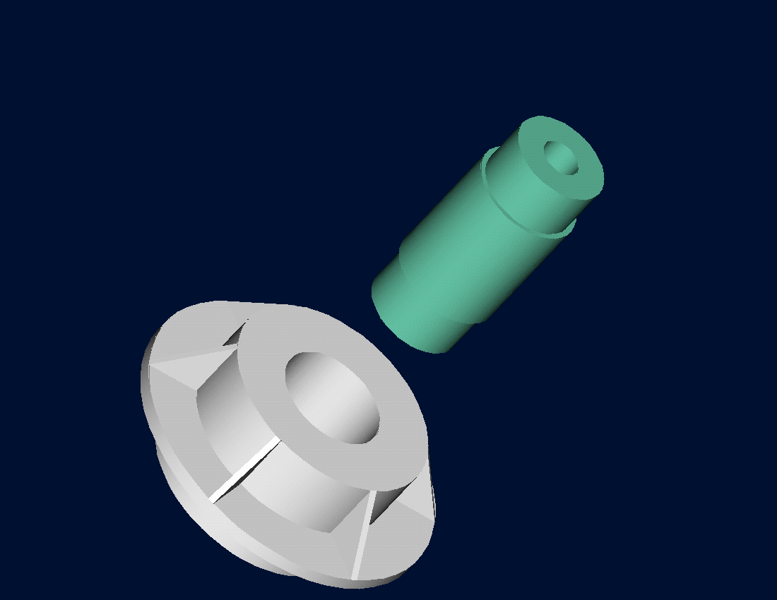
Figure 2 Trunnion slides through the hub after contracting
\[\text{Rate of heat lost due to convection} =h\left( \theta \right)A\left( \theta - \theta_{a} \right). \;\;\;\;\;\;\;\;\;\;\;\;(1)\]
where
\[h\left( \theta \right) = \text{the convective cooling coefficient,}\ \text{W/m}^{2}\cdot{\text{K}}\ \text{and is a function of temperature}\]
\[A =\text{surface area}\]
\[\theta_{a} =\text{ambient temperature of the refrigerated chamber}\]
The energy stored in the mass is given by
\[\text{Energy stored by mass} = {mC\theta}\;\;\;\;\;\;\;\;\;\;\;\;(2)\]
where
\[m = \text{mass of the trunnion,}\ \text{kg}\]
\[C = \text{specific heat of the trunnion,}\ \text{J/(kg-K)}\]
From an energy balance,
\[\begin{split} &\text{Rate at which heat is gained} - \text{Rate at which heat is lost} \\ & \text{Rate at which heat is stored} \end{split}\]
gives
\[- h\left( \theta \right)A\left( \theta - \theta_{a} \right) = mC\frac{{d\theta}}{{dt}}\;\;\;\;\;\;\;\;\;\;\;\;(3)\]
Note that the convective cooling coefficient is a function of temperature. Other material parameters such as density (affecting mass), specific heat, and thermal conductivity (affecting whether the system can be considered lumped or not) of the trunnion material are functions of temperature as well, but within our temperature range of \(27^{\circ} \text{C}\) to \(-33^{\circ} \text{C}\) these vary by only \(10\%\) from the room temperature values. So we assume these parameters to be constant.
Let us now determine the constants needed for the above ordinary differential equation.
Convection coefficient of air
The convection coefficient of air, \(h\left( \theta \right)\) is not a constant function of temperature and is given by
\[h = \frac{{Nu} \times k}{D}\;\;\;\;\;\;\;\;\;\;\;\;(4)\]
where
\[{Nu}\ \text{is the Nusselt number,}\]
\[k\ \text{is the thermal conductivity of air,}\]
\[D\ \text{is the characteristic diameter and is taken as the outer diameter of the trunnion.}\]
The Nusselt number for a vertical cylinder is given by the empirical formula [1]:
\[Nu = \left( 0.825 + \frac{0.387Ra^{\frac{1}{6}}}{\left(1+\left(\frac{0.492}{\Pr} \right)^{\frac{9}{16}} \right)^{\frac{8}{27}}}\right)^2\;\;\;\;\;\;\;\;\;\;\;\;(5)\]
where
\(Pr\) is the Prandtl number given by
\[\Pr = \frac{v_{k}}{\alpha}\;\;\;\;\;\;\;\;\;\;\;\;(6)\]
\[\nu_{k}\ \text{is the kinematic viscosity of the fluid,}\]
\[\alpha\ \text{is the thermal diffusivity,}\]
\(R_{a}\) is the Rayleigh number given by:
\[R_{a} = G_{r} \times \Pr\;\;\;\;\;\;\;\;\;\;\;\;(7)\]
\(G_{r}\) is the Grashoff number given by:
\[Gr = \frac{g\beta(T_{{wall}} - T_{{fluid}})D^{3}}{{\nu_{k}}^{2}}\;\;\;\;\;\;\;\;\;\;\;\;(8)\]
where
\[g\ \text{is the gravitational constant,}\]
\[\beta\ \text{is the coefficient of volumetric thermal expansion,}\]
\[T_{{wall}}\ \text{is the temperature of the wall,}\]
\[T_{{fluid}}\ \text{is the temperature of the fluid.}\]
To calculate the convection coefficient, we use the following value for kinematics viscosity\(\ \nu,\) thermal conductivity \(k,\) thermal diffusivity\(\ \alpha,\) and volumetric coefficient, \(\beta\) of air as a function of temperature, \(\theta\) [Ref. 1].
Table 1 Properties of air as a function of temperature.
| \(T_{lookup}\) | \(\nu\) | \(k\) | \(\alpha\) | \(\beta\) |
|---|---|---|---|---|
| \(^{\circ} C\) | \(m^2/s\) | \(W/(m-K)\) | \(m^2/s\) | \(1/K\) |
| \(-173.15\) | \(2.00 \times 10^{- 6}\) | \(9.34 \times 10^{- 3}\) | \(2.54 \times 10^{- 6}\) | \(1.00 \times 10^{- 2}\) |
| \(-123.15\) | \(4.43 \times 10^{- 6}\) | \(1.38 \times 10^{- 2}\) | \(5.84 \times 10^{- 6}\) | \(6.67 \times 10^{- 3}\) |
| \(-73.15\) | \(7.59 \times 10^{- 6}\) | \(1.81 \times 10^{- 2}\) | \(1.03 \times 10^{- 5}\) | \(5.00 \times 10^{- 3}\) |
| \(-23.15\) | \(1.14 \times 10^{- 5}\) | \(2.23 \times 10^{- 2}\) | \(1.59 \times 10^{- 5}\) | \(4.00 \times 10^{- 3}\) |
| \(26.85\) | \(1.59 \times 10^{- 5}\) | \(2.63 \times 10^{- 2}\) | \(2.25 \times 10^{- 5}\) | \(3.33 \times 10^{- 3}\) |
Other constants needed are:
\[D = 0.25\ \text{m}\]
\[g = 9.8\ \text{m/s}^{2}\]
\[T_{{fluid}} = - 33^{\circ}\text{C}\]
Table 2 Convection coefficient of air as a function of temperature.
| \(T_{wall}\) | \(T_{average}=\frac{1}{2}(T\ fluid\ +\ T\ wall)\) | \(h\) |
|---|---|---|
| \(^{\circ} C\) | \(^{\circ}C\) | \(W/(m^2.K)\) |
| \(-33\) | \(-16.50\) | \(5.846E-02\) |
| \(-18\) | \(-9.00\) | \(4.527E+00\) |
| \(-8\) | \(-4.00\) | \(5.214E+00\) |
| \(2\) | \(1.00\) | \(5.702E+00\) |
| \(27\) | \(13.50\) | \(6.533E+00\) |
The values in Table 2 are interpolated from Table 1 where temperatures are chosen as the average value for the wall and ambient temperature. The above data is interpolated as:
\[h\left( \theta \right) = - 3.69 \times 10^{- 6}\theta^{4} + 2.33 \times 10^{- 5}\theta^{3} + 1.35 \times 10^{- 3}\theta^{2} + 5.42 \times 10^{- 2}\theta + 5.59\;\;\;\;\;\;\;\;\;\;\;\;(9)\]
Area, \(A\)
\[\text{Outer radius of trunnion,}\ a = 0.125\ \text{m}.\]
\[\text{Length of trunnion,}\ L = 1.36\ \text{m}.\]
gives
\[\begin{split} A &= (2\pi a)L + 2\pi a^{2}\\ &= 2\pi\left( .125 \right)\left( 1.36 \right) + 2\pi(0.125)^{2}\\ &= 1.166\ \text{m}^{2} \end{split}\]
Mass, \(m\)
\[\text{Length of the trunnion,}\ L = 1.36\ \text{m}\]
\[\text{Density of trunnion material,}\ \rho = 7800 \text{kg/m}^3\]
gives
\[\begin{split} m &= {\rho V}\\ &=\rho(\pi r^{2}L)\\ &=7800\pi\left( 0.125 \right)^{2}1.36\\ &= 520.72\ \text{kg} \end{split}\]
Other constants
\[\text{Specific heat,}\ C = 420\ \text{J/ (kg-K)}\]
\[\text{Initial temperature of the trunnion,}\ T\left( 0 \right) = 27^{\circ} \text{C},\]
\[\text{Ambient temperature,}\ T_{a} = - 33{^\circ}\text{C}\]
The first-order ordinary differential equation:
\[- h\left( \theta \right)A\left( \theta - \theta_{a} \right) = mC\frac{{d\theta}}{{dt}}\]
reduces to
\[\begin{split} &- \left( - 3.69 \times 10^{- 6}\theta^{4} + 2.33 \times 10^{- 5}\theta^{3} + 1.35 \times 10^{- 3}\theta^{2} + 5.42 \times 10^{- 2}\theta + 5.588 \right) \times\\ &\left( 1.166 \right) \times \left( \theta + 33 \right) = \left( 520.72 \right) \times \left( 420 \right) \times \frac{{d\theta}}{{dt}}\end{split}\]
\[\frac{{d\theta}}{{dt}} = - 5.331 \times 10^{- 6}( - 3.69 \times 10^{- 6}\theta^{4} + 2.33 \times 10^{- 5}\theta^{3} + 1.35 \times 10^{- 3}\theta^{2} + 5.42 \times 10^{-2}\theta+5.588)(\theta+33)\;\;\;\;\;\;\;\;\;\;\;\;(10)\]
\[\theta\left( 0 \right) = 27{^\circ}C\]
Is the assumption of the trunnion considered as a lumped system correct?
To determine whether a system is lumped, we calculate the Biot number \(Bi\), which is defined as
\[Bi = \frac{hL}{k_{s}}\;\;\;\;\;\;\;\;\;\;\;\;(11)\]
where
\[h = \text{average surface conductance,}\]
\[L = \text{significant length dimension (volume of body/surface area),}\]
\[k_{s} = \text{thermal conductivity of solid body.}\]
If \(B_{i} < 0.1\), the temperature in the body is uniform within \(5\%\) error.
In our case:
\[h = 4.407\ \frac{\text{W}}{\text{m}^{2}\cdot{\text{K}}}\]
\[L = 1.36\ \text{m}\]
\[k_{s} = 81\ \frac{\text{W}}{\text{m}\cdot{\text{K}}}\;\;\;\;\;\;\;\;\;\;\;\;[Ref. 2]\]
\[\begin{split} Bi &= \frac{4.407 \times 1.36}{81}\\ &= 0.074 < 0.1 \end{split}\]
The Biot number is less than \(0.1\), and one can hence assume the trunnion to be a lumped mass system.
References
[1] F. B. Incropera, D. P. Dewitt, Introduction to Heat Transfer, 3rd Ed, John Wiley & Sons, Inc., New York, NY, 2000, Chap. 9.
[2] F. Kreith, M. S. Bohn, Principle of Heat Transfer, 4th Ed, Harper & Row, Publishers, New York, NY, 1993, Appendix 2.