Chapter 06.04: Nonlinear Regression
Learning Objectives
After successful completion of this lesson, you should be able to:
1) identify different nonlinear regression models,
2) recall the formula for the sum of the squares of the residuals for a general regression model.
Introduction
Many physical phenomena have a nonlinear relationship between variables. For example, unlike the linear spring you see in a weighing machine at your local grocery store in the produce section, a spring in the car’s suspension system follows a nonlinear relationship between force and its displacement. However, the fundamentals of finding the constants of nonlinear regression models are similar to what we use for linear regression modes.
The problem statement for a nonlinear regression model is still the same, that is, given \({n}\) data pairs \(\left( x_{1},y_{1} \right), \left( x_{2},y_{2} \right), \ldots, \left( x_{n},y_{n} \right)\), best fit \(y = f\left( x \right)\) to the data.
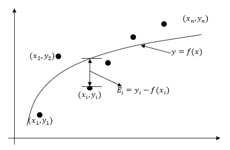
Figure 1. Nonlinear regression model for discrete \(y\) vs. \(x\) data
The residual at each data point \(x_{i}\) is found
\[E_{i} = y_{i} - f(x_{i})\;\;\;\;\;\;\;\;\;\;\;\; (1)\]
to get the sum of the square of the residuals as
\[\begin{split} S_{r} &= \sum_{i = 1}^{n}E_{i}^{2}\\ &= \sum_{i = 1}^{n}\left( y_{i} - f(x_{i}) \right)^{2}\;\;\;\;\;\;\;\;\;\;\;\; (2) \end{split}\]
Now, one minimizes the square of the residuals \(S_{r}\) with respect to the constants of the regression model \(y = f\left( x \right)\).
Common nonlinear models in science and engineering include the following.
Exponential model
Given \(\left( x_{1},y_{1} \right),\left( x_{2},y_{2} \right),\ldots,\left( x_{n},y_{n} \right)\), best fit \(y = ae^{{bx}}\) to the data. In this model, the constants of the regression model are \(a\) and \(b\). An example of the model is the case of a radioactive dye such as Technitium-99 given to patients who are going through a CT scan of their body to diagnose an illness such as excess fat on a liver. The radiation intensity of the radioactive dye decreases with time and is governed by an exponentially decaying model (Figure 2). The interest in such a model would be to find out how long substantial radiation stays in the body.

Figure 2 Relative intensity of radiation as a function of time using an exponential regression model.
Power model
Given \(\left( x_{1},y_{1} \right),\left( x_{2},y_{2} \right),\ldots,\left( x_{n},y_{n} \right)\), best fit \(y = ax^{b}\) to the data. In this model, the constants of the regression model are \(a\) and \(b\). An example of the model is a falling parachutist, where the drag force on the parachute is related through the power of the velocity with which they are falling. An interest in such a model would arise from designing the parachute such that the drag is low enough to maintain control of fall but high enough for the fall to be safe.
Saturation growth model
Given \(\left( x_{1},y_{1} \right),\ \left( x_{2},y_{2} \right), \ldots, \left( x_{n},y_{n} \right)\), best fit \(\displaystyle y = \frac{{ax}}{b + x}\) to the data. In this model, the constants of the regression model are \(a\) and \(b\). An example of the model is the case of how good animation looks. How good an animation looks is measured by a variable called performance and is a function of the frame rate. Frame rate is the frequency at which consecutive frames (images) appear on display. The higher the frame rate, the more natural animation looks to the human eye, but the human eye cannot distinguish the increased performance after a certain frame rate. This model is an example of a saturation growth model where at zero frame rate, the performance is zero as one is looking at a static image, and at high frame rates, the performance level saturates.
Harmonic decline model
Given \(\left( x_{1},y_{1} \right), \left( x_{2},y_{2} \right),\ldots,\left( x_{n},y_{n} \right)\), best fit \(\displaystyle y = \frac{b}{1 + {ax}}\) to the data. In this model, the constants of the regression model are \(a\) and \(b\). An example of the model is how much oil would be produced from a well as a function of time. An interest in such a model would arise to estimate the life of the oil well to find out when it should be abandoned.
In all the above examples, one would find the sum of the square of the residuals and minimize it with respect to the constants of the model.
For example, take the case of the exponential model. Given \(\left( x_{1},y_{1} \right), \left( x_{2},y_{2} \right),\ldots, \left( x_{n},y_{n} \right)\), best fit \(y = ae^{\text{bx}}\) to the data. The variables \(a\) and \(b\) are the constants of the exponential model. The residual at each data point \(x_{i}\) is
\[E_{i} = y_{i} - ae^{bx_{i}}\;\;\;\;\;\;\;\;\;\;\;\; (3)\]
The sum of the square of the residuals is
\[\begin{split} S_{r} &= \sum_{i = 1}^{n}E_{i}^{2}\\ &= \sum_{i = 1}^{n}\left( y_{i} - ae^{bx_{i}} \right)^{2}\;\;\;\;\;\;\;\;\;\;\;\; (4) \end{split}\]
All one must do is to minimize the sum of the square of the residuals with respect to \(a\) and \(b\). The challenge lies as the resulting equations, unlike in linear regression, turn out to be simultaneous nonlinear equations. We cover this issue in the upcoming lessons.
Learning Objectives
After successful completion of this lesson, you should be able to:
1) derive constants of nonlinear regression models using transformation of data,
2) use the derived formula to find the constants of the nonlinear regression model from given data.
Derivation of nonlinear regression models
In a previous lesson, we have discussed linear regression models. But when data is following a nonlinear trend, we need to develop nonlinear regression models. A simple example of such models is the drag force on a parachute, which is related to the square of the velocity of the parachutist. Other examples are the decay of radioactivity intensity of nuclear material, which is related exponentially to passage of time, or the height of a human that saturates as the person ages.
The derivation of the nonlinear models follows the same concept of finding the sum of the squares of the residuals and minimizing with respect to the constants of the regression model. For brevity, we limit our discussion to the exponential model in this lesson.
Exponential model
Given \(\left( x_{1},y_{1} \right),\left( x_{2},y_{2} \right),\ldots,\left( x_{n},y_{n} \right)\), best fit \(y = ae^{{bx}}\) to the data (Figure 1).
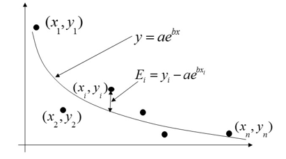
Figure 1. Exponential regression model for y vs. x data
The variables \(a\) and \(b\) are the constants of the exponential model. The residual \(E_{i}\) at each data point \(x_{i}\) is
\[E_{i} = y_{i} - ae^{bx_{i}}\;\;\;\;\;\;\;\;\;\;\;\;(1)\]
The sum of the square of the residuals is
\[\begin{split} S_{r} &= \sum_{i = 1}^{n}E_{i}^{2}\\ &= \sum_{i = 1}^{n}\left( y_{i} - ae^{bx_{i}} \right)^{2}\;\;\;\;\;\;\;\;\;\;\;\; (2) \end{split}\]
To find the constants \(a\) and \(b\) of the exponential model, we minimize \(S_{r}\) by differentiating with respect to \(a\) and \(b\) and equating the resulting equations to zero
\[\frac{\partial S_{r}}{\partial a} = \sum_{i = 1}^{n}{2\left( y_{i} - ae^{bx_{i}} \right)}\left( - e^{bx_{i}} \right) = 0\]
\[\frac{\partial S_{r}}{\partial b} = \sum_{i = 1}^{n}{2\left( y_{i} - ae^{bx_{i}} \right)}\left( - ax_{i}e^{bx_{i}} \right) = 0\;\;\;\;\;\;\;\;\;\;\;\; (3a,b)\]
Expanding Equations (3a,b) gives
\[-2\sum_{i = 1}^{n}{y_{i}e^{bx_{i}}} + 2a\sum_{i = 1}^{n}e^{2bx_{i}} = 0\]
\[-2a\sum_{i = 1}^{n}{y_{i}x_{i}e^{bx_{i}}} + 2a^2\sum_{i = 1}^{n}{x_{i}e^{2bx_{i}}} = 0\;\;\;\;\;\;\;\;\;\;\;\;(4a,b)\]
Examining the Equations (4a, b) above shows that we need to solve simultaneous nonlinear equations for the regression constants \(a\) and \(b\) and need numerical methods. Is there an alternative?
It is sometimes possible to use simple linear regression formulas to estimate the parameters of a nonlinear model. This procedure involves first transforming the given data, followed by using formulas derived for linear regression. Data for several nonlinear models such as exponential, power, and growth can be transformed, but not so for all nonlinear models.
Exponential Model through Transformation of Data
Given \(\left( x_{1},y_{1} \right),\left( x_{2},y_{2} \right),\ldots,\left( x_{n},y_{n} \right)\), best fit \(y = ae^{{bx}}\) to the data by using the transformation of data. The variables \(a\) and \(b\) are the constants of the exponential model
\[y = ae^{{bx}}\;\;\;\;\;\;\;\;\;\;\;\;(5)\]
Taking the natural log of both sides of Equation (5) gives
\[\ln y = \ln a + bx\;\;\;\;\;\;\;\;\;\;\;\;(6)\]
Let
\[z = \ln y\]
\[a_{0} = \ln a\ \text{implying}\ a = e^{a_{o}}\]
\[a_{1} = b\;\;\;\;\;\;\;\;\;\;\;\;(7)\]
then
\[z = a_{0} + a_{1}x\;\;\;\;\;\;\;\;\;\;\;\; (8)\]
For the transformed data of \(z\) versus \(x\), we can use the linear regression formulas. Hence, the constants \(a_{0}\) and \(a_{1}\) can be found as
\[a_{1} = \frac{\displaystyle n\sum_{i = 1}^{n}{x_{i}z_{i} - \sum_{i = 1}^{n}x_{i}}\sum_{i = 1}^{n}z_{i}}{\displaystyle n\sum_{i = 1}^{n}{x_{i}^{2} - \left( \sum_{i = 1}^{n}x_{i} \right)^{2}}}\]
\[a_{0} = \overset{\_}{z} - a_{1}\overset{\_}{x}\;\;\;\;\;\;\;\;\;\;\;\;(9a,b)\]
When the constants \(a_{0}\) and \(a_{1}\) are found, the original constants of the exponential model are found as given in Equation (7)
\[\begin{split} b &= a_{1}\\ a &= e^{a_{0}}\end{split}\]
Example 1
Many patients get concerned when a medical test involves an injection of radioactive material. For example, for scanning a gallbladder, a few drops of Technetium-99m isotope are used. Half of the technetium-99m would be gone in about \(6\) hours. However, it takes about \(24\) hours for the radiation levels to reach what we are exposed to in day-to-day activities. Below is given the relative intensity of radiation as a function of time.
Table 1. Relative intensity of radiation as a function of time
| \(t (hrs)\) | \(0\) | \(1\) | \(3\) | \(5\) | \(7\) | \(9\) |
|---|---|---|---|---|---|---|
| \(\gamma\) | \(1.000\) | \(0.891\) | \(0.708\) | \(0.562\) | \(0.447\) | \(0.355\) |
If the level of the relative intensity of radiation is related to time via an exponential formula \(\gamma = Ae^{{\lambda t}}\), using the transformation of data, find
a) the value of the regression constants \(A\) and \(\lambda\),
b) the half-life of Technium-99m, and
c) the radiation intensity after \(24\) hours.
Solution
a)
\[\gamma = Ae^{{\lambda t}}\;\;\;\;\;\;\;\;\;\;\;\; (E1.1)\]
Taking the natural logarithm on both sides,
\[\ln\left( \gamma \right) = \ln\left( A \right) + {\lambda t}\;\;\;\;\;\;\;\;\;\;\;\; (E1.2)\]
Assuming
\[y = \ln\gamma\]
\[a_{0} = \ln\left( A \right)\;\;\;\;\;\;\;\;\;\;\;\; (E1.3)\]
\[a_{1} = \lambda\;\;\;\;\;\;\;\;\;\;\;\; (E1.4)\]
we get
\[y = a_{0} + a_{1}t\]
This is a linear relationship between \(y\) and \(t\).Then
\[a_{1} = \frac{\displaystyle n\sum_{i = 1}^{n}{t_{i}y_{i} - \sum_{i = 1}^{n}t_{i}}\sum_{i = 1}^{n}y_{i}}{\displaystyle n\sum_{i = 1}^{n}{t_{i}^{2} - \left( \sum_{i = 1}^{n}t_{i} \right)^{2}}}\]
\[a_{0} = \bar{y} - a_{1}\bar{t}\;\;\;\;\;\;\;\;\;\;\;\;(1.5 a,b)\]
Table 2 shows the summations one would need for calculating \(a_{0}\) and \(a_{1}\).
Table 2 Summations of data to calculate constants of the model.
| \(i\) | \(t_i\) | \(y_i\) | \(y_i = ln{y_i}\) | \(t_iy_i\) | \(t_i^2\) |
|---|---|---|---|---|---|
| \(1\) | \(0\) | \(1\) | \(0.00000\) | \(0.0000\) | \(0.0000\) |
| \(2\) | \(1\) | \(0.891\) | \(-0.11541\) | \(-0.11541\) | \(1.0000\) |
| \(3\) | \(3\) | \(0.708\) | \(-0.34531\) | \(-1.0359\) | \(9.0000\) |
| \(4\) | \(5\) | \(0.562\) | \(-0.57625\) | \(-2.8813\) | \(25.0000\) |
| \(5\) | \(7\) | \(0.447\) | \(-0.80520\) | \(-5.6364\) | \(49.0000\) |
| \(6\) | \(9\) | \(0.355\) | \(-1.0356\) | \(-9.3207\) | \(81.0000\) |
| \(\displaystyle \sum_{i=1}^6\) | \(25.0000\) | \(-2.8778\) | \(-18.990\) | \(165.00\) |
\[n = 6\]
\[\sum_{i = 1}^{6}{t_{i} = 25}.000\]
\[\sum_{i = 1}^{6}{y_{i} = - 2.8778}\]
\[\sum_{i = 1}^{6}{t_{i}y_{i} = - 18.990}\]
\[\sum_{i = 1}^{6}{t_{i}^{2} = 165.00}\]
From Equation (1.5a, b) we have
\[\begin{split} a_{1} &= \frac{6\left( - 18.990 \right) - \left( 25 \right)\left( - 2.8778 \right)}{6\left( 165.00 \right) - \left( 25 \right)^{2}}\\ &= - 0.11505\end{split}\] \[\begin{split} a_{0} &= \frac{- 2.8778}{6} - \left( - 0.11505 \right)\frac{25}{6}\\ &= - 2.6150 \times 10^{- 4} \end{split}\]
Since
\[a_{0} = \ln\left( A \right)\]
\[\begin{split} A &= e^{a_{0}}\\ &= e^{- 2.6150 \times 10^{- 4}}\\ &= 0.99974\\ \end{split}\]
\[\lambda = a_{1} = - 0.11505\]
The regression formula then is
\[\gamma = 0.99974 \times e^{- 0.11505t}\]
b) Half-life is when
\[\gamma = \left. \ \frac{1}{2}\gamma \right|_{t = 0}\]
\[0.99974 \times e^{- 0.11505t} = \frac{1}{2}\left( 0.99974 \right)e^{- 0.11505\left( 0 \right)}\]
\[{e^{- 0.11508t} = 0.5 }\]
\[{- 0.11505\ t = \ln(0.5) }\]
\[{t = 6.0248\text{ hours}}\]
c) The relative intensity of radiation after \(24\) hours is
\[\begin{split} \gamma &= 0.99974e^{- 0.11505\left( 24 \right)}\\ &= 0.063200 \end{split}\]
This value of relative intensity implies that only
\[\displaystyle \frac{6.3200 \times 10^{- 2}}{0.99974} \times 100 = 6.3216\%\]
of the initial radioactivity is left after \(24\) hours.
Learning Objectives
After successful completion of this lesson, you should be able to:
1) derive constants of a nonlinear exponential regression model,
2) use the derived formula to find the constants of the exponential regression model from given data.
Nonlinear models using least squares
The development of the least-squares estimation for nonlinear models does not generally yield linear equations and hence is not easy to solve. Solving for the constants of the nonlinear models mostly results in simultaneous nonlinear equations. We illustrate this challenge through an exponential model.
Exponential model
Given \(\left( x_{1},y_{1} \right),\left( x_{2},y_{2} \right),\ldots,\left( x_{n},y_{n} \right)\), best fit \(y = ae^{{bx}}\) to the data. The variables \(a\) and \(b\) are the constants of the exponential model. The residual at each data point \(x_{i}\), is
\[E_{i} = y_{i} - ae^{bx_{i}}\;\;\;\;\;\;\;\;\;\;\;\;(1)\]
The sum of the square of the residuals is
\[\begin{split} S_{r} &= \sum_{i = 1}^{n}E_{i}^{2}\\ &= \sum_{i = 1}^{n}\left( y_{i} - ae^{bx_{i}} \right)^{2}\;\;\;\;\;\;\;\;\;\;\;\;(2) \end{split}\]
To find the constants \(a\) and \(b\) of the exponential model, we minimize \(S_{r}\) by differentiating \(S_r\) with respect to \(a\) and \(b\) and equating the resulting equations to zero
\[\frac{\partial S_{r}}{\partial a} = \sum_{i = 1}^{n}{2\left( y_{i} - ae^{bx_{i}} \right)}\left( - e^{bx_{i}} \right) = 0\]
\[\frac{\partial S_{r}}{\partial b} = \sum_{i = 1}^{n}{2\left( y_{i} - ae^{bx_{i}} \right)}\left( - ax_{i}e^{bx_{i}} \right) = 0\;\;\;\;\;\;\;\;\;\;\;\; (3a,b)\]
Expanding Equation (3a,b) gives
\[-2\sum_{i = 1}^{n}{y_{i}e^{bx_{i}}} + 2a\sum_{i = 1}^{n}e^{2bx_{i}} = 0\]
\[-2a\sum_{i = 1}^{n}{y_{i}x_{i}e^{bx_{i}}} + 2a^2\sum_{i = 1}^{n}{x_{i}e^{2bx_{i}}} = 0\;\;\;\;\;\;\;\;\;\;\;\;(4a,b)\]
Simplifying Equation (4a,b) gives
\[-\sum_{i = 1}^{n}{y_{i}e^{bx_{i}}} + a\sum_{i = 1}^{n}e^{2bx_{i}} = 0\]
\[-\sum_{i = 1}^{n}{y_{i}x_{i}e^{bx_{i}}} + a\sum_{i = 1}^{n}{x_{i}e^{2bx_{i}}} = 0\;\;\;\;\;\;\;\;\;\;\;\;(5a,b)\]
Equations (5a) and (5b) are nonlinear in \(a\) and \(b\) and thus not in a closed-form to be solved as was the case for linear regression. In general, iterative methods (such as Gauss‑Newton iteration method, method of steepest descent, Marquardt’s method, direct search, etc) must be used to find values of \(a\) and \(b\).
However, in this case, from Equation (5a), \({a}\) can be written explicitly in terms of \({b}\) as
\[a = \frac{\displaystyle \sum_{i = 1}^{n}{y_{i}e^{bx_{i}}}}{\displaystyle \sum_{i = 1}^{n}e^{2bx_{i}}}\;\;\;\;\;\;\;\;\;\;\;\;(6)\]
Substituting Equation (6) in (5b) gives
\[\sum_{i = 1}^{n}y_{i}x_{i}e^{bx_{i}} - \frac{\displaystyle \sum_{i = 1}^{n}y_{i}e^{bx_{i}}}{\displaystyle \sum_{i = 1}^{n}e^{2bx_{i}}}\sum_{i = 1}^{n}{x_{i}e^{2bx_{i}}} = 0\;\;\;\;\;\;\;\;\;\;\;\;(7)\]
This equation is still nonlinear in \(b\) and can be solved best by numerical methods such as the bisection method or the secant method.
Example 1
Many patients get concerned when a test involves an injection of radioactive material. For example, for scanning a gallbladder, a few drops of Technetium-99m isotope are used. Half of the technetium-99m would be gone in about 6 hours. It, however, takes about 24 hours for the radiation levels to reach what we are exposed to in day-to-day activities. Below is given the relative intensity of radiation as a function of time.
Table 1 Relative intensity of radiation as a function of time
| \(t\left( \text{hrs} \right)\) | \(0\) | \(1\) | \(3\) | \(5\) | \(7\) | \(9\) |
|---|---|---|---|---|---|---|
| \(\gamma\) | \(1.000\) | \(0.891\) | \(0.708\) | \(0.562\) | \(0.447\) | \(0.355\) |
If the level of the relative intensity of radiation is related to time via an exponential formula \(\gamma = Ae^{{\lambda t}}\), find
a). the value of the regression constants \(A\) and \(\lambda\),
b). the half-life of Technium-99m, and
c). the radiation intensity after \(24\) hours.
Solution
a) The value of \(\lambda\) is given by solving the nonlinear Equation (7),
\[f\left( \lambda \right) = \sum_{i = 1}^{n}\gamma_{i}t_{i}e^{\lambda t_{i}} - \frac{\displaystyle \sum_{i = 1}^{n}{\gamma_{i}e^{\lambda t_{i}}}}{\displaystyle \sum_{i = 1}^{n}e^{2\lambda t_{i}}}\sum_{i = 1}^{n}{t_{i}e^{2\lambda t_{i}}} = 0\;\;\;\;\;\;\;\;\;\;\;\;(E1.1)\]
Then the value of \(A\) from Equation (6) takes the form,
\[A = \frac{\displaystyle \sum_{i = 1}^{n}{\gamma_{i}e^{\lambda t_{i}}}}{\displaystyle \sum_{i = 1}^{n}e^{2\lambda t_{i}}}\;\;\;\;\;\;\;\;\;\;\;\;(E1.2)\]
Equation (E1.1) can be solved for \(\lambda\) using the bisection method. To estimate the initial guesses, we assume \(\lambda = - {0.120}\) and \(\lambda = - {0.110}\). We need to check whether these values first bracket the root of \(f\left( \lambda \right) = 0\). At \(\lambda = - {0.120}\), the table below shows the evaluation of \(f\left( - {0.120} \right)\).
Table 2 Summation value for calculation of constants of the model
| \(i\) | \(t_{i}\) | \(\gamma_{i}\) | \(\gamma_{i} t_{i} e^{\lambda t_{i}}\) | \(\gamma_{i} e^{\lambda t_{i}}\) | \(e^{2 \lambda t_{i}}\) | \(t_{i} e^{2 \lambda t_{i}}\) |
|---|---|---|---|---|---|---|
\(1\) \(2\) \(3\) \(4\) \(5\) \(6\) |
\(0\) \(1\) \(3\) \(5\) \(7\) \(9\) |
\(1\) \(0.891\) \(0.708\) \(0.562\) \(0.447\) \(0.355\) |
\(0.00000\) \(0.79205\) \(1.4819\) \(1.5422\) \(1.3508\) \(1.0850\) |
\(1.00000\) \(0.79205\) \(0.49395\) \(0.30843\) \(0.19297\) \(0.12056\) |
\(1.00000\) \(0.78663\) \(0.48675\) \(0.30119\) \(0.18637\) \(0.11533\) |
\(0.00000\) \(0.78663\) \(1.4603\) \(1.5060\) \(1.3046\) \(1.0379\) |
| \(\displaystyle \sum_{i=1}^{6}\) | \(6.2501\) | \(2.9062\) | \(2.8763\) | \(6.0954\) |
From Table 2
\[n = 6\]
\[\sum_{i = 1}^{6}\gamma_{i}t_{i}e^{- 0.120t_{i}} = 6.2501\]
\[\sum_{i = 1}^{6}\gamma_{i}e^{- 0.120t_{i}} = 2.9062\]
\[\sum_{i = 1}^{6}e^{2\left( - 0.120 \right)t_{i}} = 2.8763\]
\[\sum_{i = 1}^{6}t_{i}e^{2\left( - 0.120 \right)t_{i}} = 6.0954\]
\[\begin{split} f\left( - 0.120 \right) &= \left( 6.2501 \right) - \frac{2.9062}{2.8763}\left( 6.0954 \right)\\ &= 0.091357 \end{split}\]
Similarly
\[f\left( - 0.110 \right) = - 0.10099\]
Since
\[f\left( - 0.120 \right) \times f\left( - 0.110 \right) < 0,\]
the value of \(\lambda\) falls in the bracket of \(\left\lbrack - {0.120,} - {0.110} \right\rbrack\). The next guess of the root then is
\[\begin{split} \lambda &= \frac{- 0.120 + \left( - 0.110 \right)}{2}\\ &= - 0.115 \end{split}\]
Continuing with the bisection method, the root of \(f\left( \lambda \right) = 0\) is found as \(\lambda = - 0.11508\). This value of the root was obtained after 20 iterations with an absolute relative approximate error of less than \(0.000008\%\).
From Equation (E1.2), \(A\) can be calculated as
\[\begin{split} A &= \frac{\displaystyle \sum_{i = 1}^{6}{\gamma_{i}e^{\lambda t_{i}}}}{\displaystyle \sum_{i = 1}^{6}e^{2\lambda t_{i}}}\\ &= \frac{\begin{matrix} 1 \times e^{- 0.11508\left( 0 \right)} + 0.891 \times e^{- 0.11508\left( 1 \right)} + 0.708 \times e^{- 0.11508\left( 3 \right)} + \\ 0.562 \times e^{- 0.11508\left( 5 \right)} + 0.447 \times e^{- 0.11508\left( 7 \right)} + 0.355 \times e^{- 0.11508\left( 9 \right)} \\ \end{matrix}}{\begin{matrix} e^{2\left( - 0.11508 \right)\left( 0 \right)} + e^{2\left( - 0.11508 \right)\left( 1 \right)} + e^{2\left( - 0.11508 \right)\left( 3 \right)} + \\ e^{2\left( - 0.11508 \right)\left( 5 \right)} + e^{2\left( - 0.11508 \right)\left( 7 \right)} + e^{2\left( - 0.11508 \right)\left( 9 \right)} \\ \end{matrix}}\\ &= \frac{2.9373}{2.9378}\\ &= 0.99983 \end{split}\]
The regression formula is hence given by
\[\gamma = 0.99983\ e^{- 0.11508t}\]
b) Half-life of Technetium-99m is when
\[\displaystyle \gamma = \left. \ \frac{1}{2}\gamma \right|_{t = 0}\]
\[0.99983 \times e^{-0.11508 t}=\frac{1}{2}(0.99983) e^{-0.11508(0)}\]
\[e^{-0.11508 t}=0.5\]
\[-0.11508 t=\ln (0.5)\]
\[t=6.0232 \text{ hours }\]
c) The relative intensity of the radiation after \(24\) hours is
\[\begin{split} \gamma &= 0.99983 \times e^{- 0.11508\left( 24 \right)}\\ &= 6.3160 \times 10^{- 2} \end{split}\]
This value of relative intensity implies that only
\[\displaystyle \frac{6.3160 \times 10^{- 2}}{0.99983} \times 100 = 6.3171\%\]
of the initial radioactivity is left after \(24\) hours.
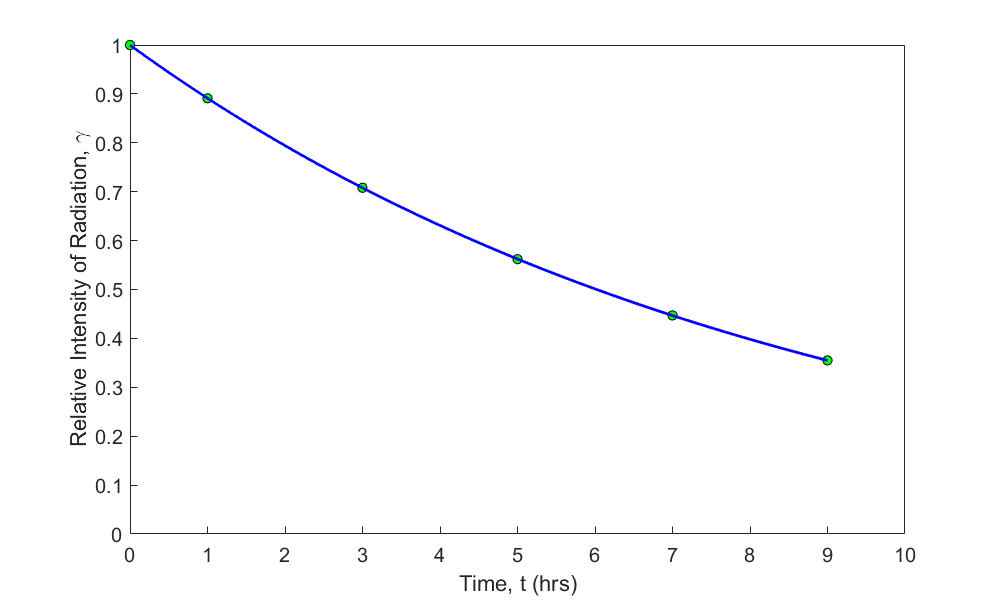
Figure 1 Relative intensity of radiation as a function of time using an exponential regression model.
How different are the constants of the model when compared to when the data is transformed?
The regression formula obtained without transforming the data is
\[\gamma = 0.99983\ e^{- 0.11508t}\]
and the regression formula obtained with transforming the data is
\[\gamma = 0.99974 e^{- 0.11505t}\]
Such proximity of the constants of the model for this example may lead us to believe that it does not matter much whether we transform the data or not. Far from it, as we will see in the next example.
Example 2
Given the data below, regress the data to \(y = e^{{bx}}\) with and without data transformation.
| \(x\) | \(y\) |
|---|---|
| \(0\) | \(1.0000\) |
| \(5\) | \(0.8326\) |
| \(10\) | \(0.6738\) |
| \(15\) | \(0.5837\) |
| \(20\) | \(0.5150\) |
| \(25\) | \(0.4163\) |
| \(40\) | \(0.3219\) |
| \(60\) | \(0.2466\) |
| \(90\) | \(0.1803\) |
Solution
Regress \(\left( x_{1},y_{1} \right),\left( x_{2},y_{2} \right),\ldots,\left( x_{n},y_{n} \right)\) data to
\[y = e^{{bx}}\;\;\;\;\;\;\;\;\;\;\;\;(E2.1)\]
regression model.
Transforming the data
The value of b can be found by transforming the data by taking the natural log of both sides of the model equation as
\[\ln(y) = \ln(e^{{bx}})\;\;\;\;\;\;\;\;\;\;\;\; (E2.2)\]
\[\ln\left( y \right) = bx\;\;\;\;\;\;\;\;\;\;\;\;(E2.3)\]
Assuming
\[z = \ln y\;\;\;\;\;\;\;\;\;\;\;\;(E2.4)\]
We get a special linear model (intercept is zero) relating the z data to x,
\[z = bx\;\;\;\;\;\;\;\;\;\;\;\;(E2.5)\]
and this linear model on minimizing the sum of the squares of the residuals gives
\[b = \frac{\displaystyle \sum_{i = 1}^{n}{x_{i}\ln(y_{i})}}{\displaystyle \sum_{i = 1}^{n}x_{i}^{2}}\;\;\;\;\;\;\;\;\;\;\;\;(E2.6)\]
Substituting the values of the data points gives
\[\sum_{i = 1}^{9}{x_{i}\ln(y_{i})} = - 331.64\]
\[\sum_{i = 1}^{n}{x_{i}^{2} = 14675}\]
\[\begin{split} b &= \frac{- 331.64}{14675}\\ &= - 0.02260 \end{split}\]
The regression model obtained with transforming the data is hence given by
\[y=e^{-0.02260x}\]
Without transforming the data
Here we need to start from the sum of the square of the residuals of the original model (Equation E2.1), and minimize the sum with respect to b. The residual is given by
\[E_{i} = y_{i} - ae^{bx_{i}}\;\;\;\;\;\;\;\;\;\;\;\;(E2.7)\]
The sum of the square of the residuals is
\[\begin{split} S_{r} &= \sum_{i = 1}^{n}E_{i}^{2}\\ &= \sum_{i = 1}^{n}\left( y_{i} - e^{bx_{i}} \right)^{2}\;\;\;\;\;\;\;\;\;\;\;\; (E2.8) \end{split}\]
To find the constant \(b\) of the exponential model, we minimize \(S_{r}\) by differentiating with respect to \(b\) and equating the resulting expression to zero
\[\frac{dS_{r}}{{db}} = \sum_{i = 1}^{n}{2\left( y_{i} - e^{bx_{i}} \right)}\left( - x_{i}e^{bx_{i}} \right) = 0\;\;\;\;\;\;\;\;\;\;\;\;(E2.9)\]
Expanding and simplifying Equation (E2.9) gives
\[\sum_{i = 1}^{n}{( - y}_{i}x_{i}e^{bx_{i}} + x_{i}e^{2bx_{i}}) = 0\]
This is a nonlinear equation in terms of \(b\), and can be solved by numerical methods such as bisection method. The value of \(b\) obtained is
\[b = - 0.03071\]
From the above solution, the regression formula obtained without transforming the data is
\[y = e^{- 0.03071x}\]
The regression formula obtained with transforming the data is
\[y = \ e^{- 0.02260x}\]
Clearly, the two models are not close, and you can see this in Figure 2 as well.
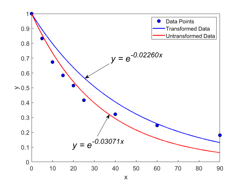
Figure 2. Comparing an exponential regression model with and without data transformation
Learning Objectives
After successful completion of this lesson, you should be able to:
1) derive formulas for the regression constants of a polynomial regression model
2) apply the polynomial regression model to given data.
Polynomial Models
Given \(n\) data points \((x_{1},y_{1}),(x_{2},y_{2}),......,(x_{n},y_{n}),\) use the least-squares method to regress the data to an \(m^{th}\) order polynomial.
\[y = a_{0} + a_{1}x + a_{2}x^{2} + \cdots\cdots + a_{m}x^{m},\ m < n \;\;\;\;\;\;\;\;\;\;\;\; (1)\]
The residual at each data point is given by
\[E_{i} = y_{i} - a_{0} - a_{1}x_{i} - ... - a_{m}x_{i}^{m}\;\;\;\;\;\;\;\;\;\;\;\; (2)\]
The sum of the square of the residuals is given by
\[\begin{split} S_{r} &= \sum_{i = 1}^{n}E_{i}^{2}\\ &= \sum_{i = 1}^{n}\left( y_{i} - a_{0} - a_{1}x_{i} - ... - a_{m}x_{i}^{m} \right)^{2}\;\;\;\;\;\;\;\;\;\;\;\; (3) \end{split}\]
To find the constants of the polynomial regression model, we put the derivatives with respect to \(a_{i},\ i=1,2,\ldots,m\) to zero, that is,
\[\begin{split} \frac{\partial S_{r}}{\partial a_{0}} &= \sum_{i = 1}^{n}{2\left( y_{i} - a_{0} - a_{1}x_{i} - ... - a_{m}x_{i}^{m} \right)}( - 1) = 0\\ \frac{\partial S_{r}}{\partial a_{1}} &= \sum_{i = 1}^{n}{2\left( y_{i} - a_{0} - a_{1}x_{i} - ... - a_{m}x_{i}^{m} \right)}( - x_{i}) = 0\\ \vdots\ \ \ \ &= \ \ \ \vdots \\ \frac{\partial S_{r}}{\partial a_{m}} &= \sum_{i = 1}^{n}{2\left( y_{i} - a_{0} - a_{1}x_{i} - ... - a_{m}x_{i}^{m} \right)}( - x_{i}^{m}) = 0 \end{split}\]
Setting these equations in matrix form gives
\[\begin{bmatrix} n & \left( \displaystyle \sum_{i = 1}^{n}x_{i} \right) & {...}\left( \displaystyle \sum_{i = 1}^{n}x_{i}^{m} \right) \\ \left( \displaystyle \sum_{i = 1}^{n}x_{i} \right) & \left( \displaystyle \sum_{i = 1}^{n}x_{i}^{2} \right) & {...}\left( \displaystyle \sum_{i = 1}^{n}x_{i}^{m + 1} \right) \\ \begin{matrix} ... \\ \left( \displaystyle \sum_{i = 1}^{n}x_{i}^{m} \right) \\ \end{matrix} & \begin{matrix} ... \\ \left( \displaystyle \sum_{i = 1}^{n}x_{i}^{m + 1} \right) \\ \end{matrix} & \begin{matrix} .... \\ ...\left( \displaystyle \sum_{i = 1}^{n}x_{i}^{2m} \right) \\ \end{matrix} \\ \end{bmatrix}\begin{bmatrix} a_{0} \\ a_{1} \\ ... \\ a_{m} \\ \end{bmatrix} = \begin{bmatrix} \displaystyle \sum_{i = 1}^{n}y_{i} \\ \displaystyle \sum_{i = 1}^{n}{x_{i}y_{i}} \\ \begin{matrix} ... \\ \displaystyle \sum_{i = 1}^{n}{x_{i}^{m}y_{i}} \\ \end{matrix} \\ \end{bmatrix}\;\;\;\;\;\;\;\;\;\;\;\; (4)\]
The above equations are solved for \(a_{0},a_{1},...,a_{m}\).
Example 1
To find the contraction of a steel cylinder, one wishes to regress the coefficient of linear thermal expansion data to temperature.
Table 1 Coefficient of linear thermal expansion at given different temperatures
| Temperature, \(T\) \((^{\circ}\text{F})\) | Coefficient of thermal expansion, \(\alpha(\text{in/in/}^{\circ}\text{F})\) |
|---|---|
| \(80\) | \(6.47 \times 10^{- 6}\) |
| \(40\) | \(6.24 \times 10^{- 6}\) |
| \(-40\) | \(5.72 \times 10^{- 6}\) |
| \(-120\) | \(5.09 \times 10^{- 6}\) |
| \(-200\) | \(4.30 \times 10^{- 6}\) |
| \(-280\) | \(3.33 \times 10^{- 6}\) |
| \(-340\) | \(2.45 \times 10^{- 6}\) |
Regress the above data to \(\alpha = a_{0} + a_{1}T + a_{2}T^{2}\)
Solution
Since \(\alpha = a_{0} + a_{1}T + a_{2}T^{2}\) is the quadratic relationship between the coefficient of linear thermal expansion and the temperature, the coefficients \(a_{0},\ a_{1},\ a_{2}\) are found as follows
\[\displaystyle \begin{bmatrix} n & \left( \displaystyle \sum_{i = 1}^{n}T_{i} \right) & \left( \displaystyle \sum_{i = 1}^{n}T_{i}^{2} \right) \\ \left( \displaystyle \sum_{i = 1}^{n}T_{i} \right) & \left( \displaystyle \sum_{i = 1}^{n}T_{i}^{2} \right) & \left( \displaystyle \sum_{i = 1}^{n}T_{i}^{3} \right) \\ \left( \displaystyle \sum_{i = 1}^{n}T_{i}^{2} \right) & \left( \displaystyle \sum_{i = 1}^{n}T_{i}^{3} \right) & \left( \displaystyle \sum_{i = 1}^{n}T_{i}^{4} \right) \\ \end{bmatrix}\begin{bmatrix} \ a_{0} \\ \ a_{1} \\ \ a_{2} \\ \end{bmatrix} = \begin{bmatrix} \displaystyle \sum_{i = 1}^{n}\alpha_{i} \\ \displaystyle \sum_{i = 1}^{n}{T_{i}\alpha_{i}} \\ \displaystyle \sum_{i = 1}^{n}{T_{i}^{2}{\alpha_{i}}^{}} \\ \end{bmatrix}\;\;\;\;\;\;\;\;\;\;\;\; (E1.1)\]
Table 2 Summations for calculating constants of the model
| \(i\) | \(T(^{\circ}\text{F})\) | \(\alpha(\text{in/in/}^{\circ}\text{F})\) | \(T^2\) | \(T^3\) |
|---|---|---|---|---|
| \(1\) | \(80\) | \(6.4700 \times 10^{- 6}\) | \(6.4000 \times 10^{3}\) | \(5.1200 \times 10^{5}\) |
| \(2\) | \(40\) | \(6.2400 \times 10^{- 6}\) | \(1.6000 \times 10^{3}\) | \(6.4000 \times 10^{4}\) |
| \(3\) | \(-40\) | \(5.7200 \times 10^{- 6}\) | \(1.6000 \times 10^{3}\) | \(- 6.4000 \times 10^{4}\) |
| \(4\) | \(-120\) | \(5.0900 \times 10^{- 6}\) | \(1.4400 \times 10^{4}\) | \(- 1.7280 \times 10^{6}\) |
| \(5\) | \(-200\) | \(4.3000 \times 10^{- 6}\) | \(4.0000 \times 10^{4}\) | \(- 8.0000 \times 10^{6}\) |
| \(6\) | \(-280\) | \(3.3300 \times 10^{- 6}\) | \(7.8400 \times 10^{4}\) | \(- 2.1952 \times 10^{7}\) |
| \(7\) | \(-340\) | \(2.4500 \times 10^{- 6}\) | \(1.1560 \times 10^{5}\) | \(- 3.9304 \times 10^{7}\) |
| \(\displaystyle \sum_{i = 1}^{7}{}\) | \(- 8.6000 \times 10^{2}\) | \(3.3600 \times 10^{- 5}\) | \(2.5800 \times 10^{5}\) | \(- 7.0472 \times 10^{7}\) |
Table 2 (cont)
| \(i\) | \(T^{4}\) | \(T \times \alpha\) | \(T^{2} \times \alpha\) |
|---|---|---|---|
| \(1\) | \(4.0960 \times 10^{7}\) | \(5.1760 \times 10^{- 4}\) | \(4.1408 \times 10^{- 2}\) |
| \(2\) | \(2.5600 \times 10^{6}\) | \(2.4960 \times 10^{- 4}\) | \(9.9840 \times 10^{- 3}\) |
| \(3\) | \(2.5600 \times 10^{6}\) | \(- 2.2880 \times 10^{- 4}\) | \(9.1520 \times 10^{- 3}\) |
| \(4\) | \(2.0736 \times 10^{8}\) | \(- 6.1080 \times 10^{- 4}\) | \(7.3296 \times 10^{- 2}\) |
| \(5\) | \(1.6000 \times 10^{9}\) | \(- 8.6000 \times 10^{- 4}\) | \(1.7200 \times 10^{- 1}\) |
| \(6\) | \(6.1466 \times 10^{9}\) | \(- 9.3240 \times 10^{- 4}\) | \(2.6107 \times 10^{- 1}\) |
| \(7\) | \(1.3363 \times 10^{10}\) | \(- 8.3300 \times 10^{- 4}\) | \(2.8322 \times 10^{- 1}\) |
| \(\displaystyle \sum_{i = 1}^{7}{}\) | \(2.1363 \times 10^{10}\) | \(- 2.6978 \times 10^{- 3}\) | \(8.5013 \times 10^{- 1}\) |
\[n = 7\] \[\sum_{i = 1}^{7}T_{i} = - 8.6000 \times 10^{- 2}\] \[\sum_{i = 1}^{7}T_{i}^{2} = 2.5580 \times 10^{5}\] \[\sum_{i = 1}^{7}T_{i}^{3} = - 7.0472 \times 10^{7}\] \[\sum_{i = 1}^{7}T_{i}^{4} = 2.1363 \times10^{10}\] \[\sum_{i = 1}^{7}{\alpha_{i}} = 3.3600 \times 10^{- 5}\] \[\sum_{i = 1}^{7}{T_{i}\alpha_{i} } = - 2.6978 \times 10^{- 3}\] \[\sum_{i = 1}^{7}{T_{i}^{2}\alpha_{i}} = \ 8.5013 \times 10^{- 1}\]
From Equation (E1.1), we have
\[\begin{bmatrix} 7.0000 & - 8.6000 \times 10^{2} & 2.5800 \times 10^{5} \\ - 8.600 \times 10^{2} & 2.5800 \times 10^{5} & - 7.0472 \times 10^{7} \\ 2.5800 \times 10^{5} & - 7.0472 \times 10^{7} & 2.1363 \times 10^{10} \\ \end{bmatrix}\begin{bmatrix} a_{0} \\ a_{1} \\ a_{2} \\ \end{bmatrix} = \begin{bmatrix} 3.3600 \times 10^{- 5} \\ - 2.6978 \times 10^{- 3} \\ 8.5013 \times 10^{- 1} \\ \end{bmatrix}\]
Solving the above system of simultaneous linear equations, we get
\[\begin{bmatrix} a_{0} \\ a_{1} \\ a_{2} \\ \end{bmatrix} = \begin{bmatrix} 6.0217 \times 10^{- 6} \\ 6.2782 \times 10^{- 9} \\ - 1.2218 \times 10^{- 11} \\ \end{bmatrix}\]
The polynomial regression model hence is
\[\displaystyle \begin{split} \alpha &= a_{0} + a_{1}T + a_{2}T^{2}
\\ &= 6.0217 \times {1}{0}^{- 6} + {6.2782} \times {1} {0}^{- 9}T - {1.2218} \times {1}{0}^{- {11}}T^{2} \end{split}\]
Learning Objectives
After successful completion of this lesson, you should be able to:
1) Choose an optimum order of polynomial for polynomial regression models.
Introduction
Often, you may not have the privilege or enough knowledge of the problem to choose the type of regression model. Some may suggest fitting the data to a polynomial model. But the question that you would begin to ask then is \(-\) What order of polynomial should I use?
Say, if you are given \(n\) data points, \((x_{1},y_{1}),(x_{2},y_{2}),......,(x_{n},y_{n})\), you could use the least-squares method to regress the data to an \(m^{th}\) order polynomial, where the order, \(m\) can be as low as \(0\) and as high as \(n - 1\).
\[y = a_{0} + a_{1}x + a_{2}x^{2} + \cdots\cdots + a_{m}x^{m},\ 0 \leq m \leq n - 1\;\;\;\;\;\;\;\;\;\;\;\; (1)\]
Look at Figures 1 and 2, where the data from Table 1, which has 22 data points, has been regressed to a first-order and second-order polynomial.
Table 1 Instantaneous thermal expansion coefficient as a function of temperature for steel
| Temperature | Instantaneous Thermal Expansion |
|---|---|
| \({^\circ}\text{F}\) | \(\mu \text{in/in/} ^{\circ}\text{F}\) |
| \(80\) | \(6.47\) |
| \(60\) | \(6.36\) |
| \(40\) | \(6.24\) |
| \(20\) | \(6.12\) |
| \(0\) | \(6.00\) |
| \(-20\) | \(5.86\) |
| \(-40\) | \(5.72\) |
| \(-60\) | \(5.58\) |
| \(-80\) | \(5.43\) |
| \(-100\) | \(5.28\) |
| \(-120\) | \(5.09\) |
| \(-140\) | \(4.91\) |
| \(-160\) | \(4.72\) |
| \(-180\) | \(4.52\) |
| \(-200\) | \(4.30\) |
| \(-220\) | \(4.08\) |
| \(-240\) | \(3.83\) |
| \(-260\) | \(3.58\) |
| \(-280\) | \(3.33\) |
| \(-300\) | \(3.07\) |
| \(-320\) | \(2.76\) |
| \(-340\) | \(2.45\) |
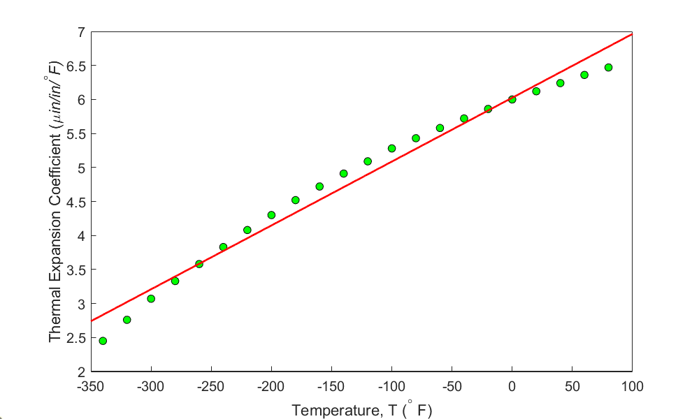
Figure 1(a) Polynomial regression model \(\alpha = 0.009387T + 6.025\) for the linear coefficient of thermal expansion vs. temperature data for steel.
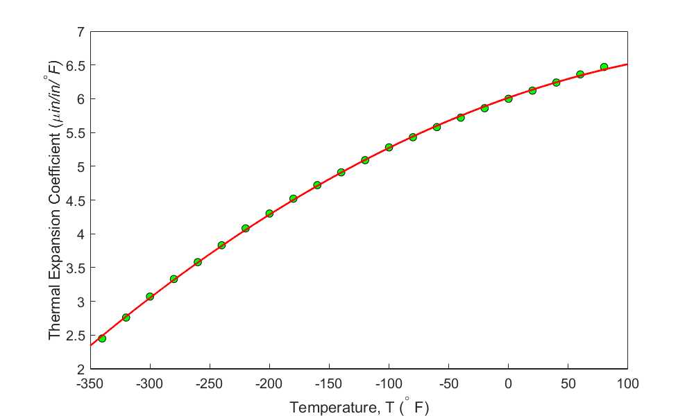
Figure 1(b). Polynomial regression model \(\alpha = - 0.000012{28T}^{2} + 0.006196T + 6.015\) for the linear coefficient of thermal expansion vs. temperature data for steel.
Visual observation of Figure 1(b) may make us believe that the second-order polynomial looks acceptable. However, we should be basing such decisions on quantitative measurements as we may not have the luxury of a visual inspection. Even if we did, the visual interpretation is speculative.
One may hence suggest using a polynomial order for which the sum of the squares of the residuals, \(S_{r}\) is a minimum. For the data in Table 1, the sum of the square of the residuals, \(S_{rm}\) as a function of the order of the polynomial, \(m\) is shown in Table 2, Figure (2a), and Figure (2b).
Table 2.
| \(\text{Order of polynomial},\) \({m}\) | \({S_{rm}}\) |
|---|---|
| \(1\) | \(0.6912\) |
| \(2\) | \(0.007732\) |
| \(3\) | \(0.001063\) |
| \(4\) | \(0.001013\) |
| \(5\) | \(0.0009019\) |
| \(6\) | \(0.0006700\) |
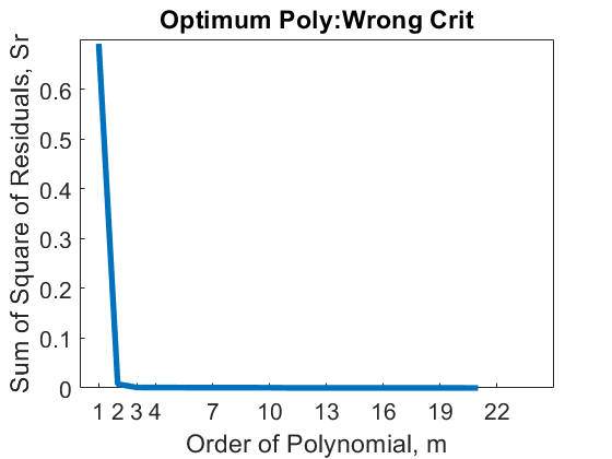
Figure 2(a): Sum of square of residuals as a function of the order of the polynomial. This graph starts at \(m = 1\)
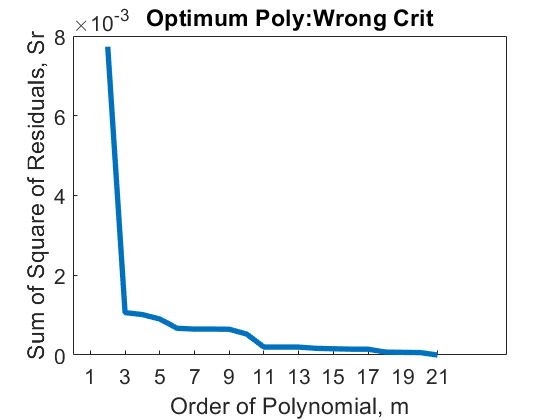
Figure 2(b): Sum of square of residuals as a function of the order of the polynomial. This graph is the same as Figure 2(a) but starts at \(m = 2\)
The value of \(S_{rm}\) continues to decrease with the increase in the order of the polynomial (Figures 2a and 2b), and in fact, we will get \(S_{rm} = 0\) when the chosen polynomial order is one less than the number of data points (of course, we assume there is only one y-value for each x-value). In this case, the regression curve would go through all the points and be a perfect fit. In fact, it is polynomial interpolation for this extreme case. Using the criterion of minimizing \(S_{{rm}}\) with respect to the order of the polynomial is hence not acceptable.
Instead, the criterion suggested to use is as follows. Given \((x_{1},y_{1}),(x_{2},y_{2}),\ldots\ldots,(x_{n},y_{n})\) data points, choose the degree of the polynomial, \(m\) for which the variance as computed by
\[\text {Variance} = \frac{S_{rm}}{n - (m + 1)}\;\;\;\;\;\;\;\;\;\;\;\; (2)\]
is a minimum or when there is no statistically significant decrease in its value as the degree of the polynomial is increased, where
\[S_{{rm}} = \text{sum of the square of the residuals} \text{ for the polynomial of order,}\ m.\]
Note the reason \(m + 1\) is in the formula, as there are as many constants in the polynomial regression model of order, \(m\). Also, \(S_{{rm}} = 0\), when \(n = m + 1.\) As the order of the polynomial, \(m\) increases, both the numerator, \(S_{rm},\) and the denominator, \(n - (m + 1),\) decrease. These competing decreases would allow us to optimize the order of the polynomial.
For the data in Table 1, the variance is shown as a function of the order of the polynomial in Table 3 (shown only up to \(m\)=6), and Figures (3a) and (3b).
Table 3 Variance as a function of the order of the polynomial.
| \(\text{Order of polynomial,}\) \({m}\) | \({\frac{S_{rm}}{n - (m + 1)}}\) |
|---|---|
| \(1\) | \(0.03455\) |
| \(2\) | \(0.0004069\) |
| \(3\) | \(0.00005906\) |
| \(4\) | \(0.00005961\) |
| \(5\) | \(0.00005637\) |
| \(6\) | \(0.00004467\) |
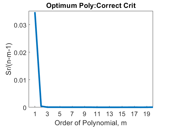
Figure 3(a): Variance as a function of the order of the polynomial. This graph starts at \(m = 1\)
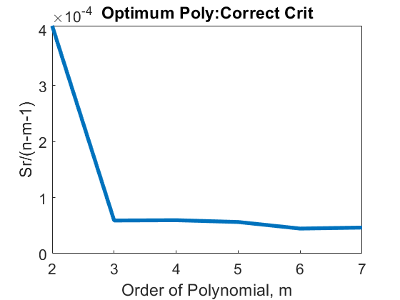
Figure 3(b): Sum of square of residuals as a function of the order of the polynomial. This graph is the same as Figure 3(a) but starts at \(m = 2\)
So, what order of polynomial would you choose? A second- or third-order polynomial would be the right choice as little statistical change occurs in the variance value after \(m = 2\).
Learning Objectives
After successful completion of this lesson, you should be able to:
1) derive constants of other popular nonlinear regression models
2) use the derived formula to find the constants of nonlinear regression models from given data with and without transformation.
Introduction
In the previous lessons, we talked about several nonlinear regression models, such as exponential. In this lesson, we continue our discussion on some growth and power regression models.
Growth model
Common growth models standard in scientific fields have been developed and are used successfully for specific situations. The growth models are used to describe how something grows with changes in the regressor variable (often the time). Examples in this category include the growth of thin films or population with time and are of the form
\[y = \frac{a}{1 + be^{- {cx}}} \;\;\;\;\;\;\;\;\;\;\;\; (1)\]
where \(a,\ b\) and \(c\) are the constants of the model.
At \(x = 0\), \(\displaystyle y = \frac{a}{1 + b}\) and
as \(x \rightarrow \infty\), \(y \rightarrow a\).
The residuals at each data point \(x_{i}\), are
\[E_{i} = y_{i} - \frac{a}{1 + be^{- cx_{i}}}\;\;\;\;\;\;\;\;\;\;\;\; (2)\]
The sum of the square of the residuals is
\[\begin{split} S_{r} &= \sum_{i = 1}^{n}E_{i}^{2}\\ &= {\sum_{i = 1}^{n}\left( y_{i} - \frac{a}{1 + be^{- cx_{i}}} \right)}^{2}\ (3) \end{split}\]
To find the constants \(a\), \(b\), and \(c,\) we minimize \(S_{r}\) by differentiating \(S_r\) with respect to \(a\), \(b\) and \(c\), and equating the resulting equations to zero.
\[\frac{\partial S_{r}}{\partial a} = \sum_{i = 1}^{n}\left( \frac{2e^{cx_{i}}\left\lbrack ae^{cx_{i}} - y_{i}\left( e^{cx_{i}} + b \right) \right\rbrack}{\left( e^{cx_{i}} + b \right)^{2}} \right) = 0,\] \[\frac{\partial S_{r}}{\partial b} = \sum_{i = 1}^{n}\left( \frac{2ae^{cx_{i}}\left\lbrack by_{i} + e^{cx_{i}}\left( y_{i} - a \right) \right\rbrack}{\left( e^{cx_{i}} + b \right)^{3}} \right) = 0,\] \[\frac{\partial S_{r}}{\partial c} = \sum_{i = 1}^{n}\left(\frac{- 2{ab}x_{i}e^{cx_{i}}\left\lbrack by_{i} + e^{cx_{i}}\left( y_{i} - a \right) \right\rbrack}{\left( e^{cx_{i}} + b \right)^{3}} \right) = 0. \;\;\;\;\;\;\;\;\;\;\;\; (4a,b,c)\]
One can use the Newton-Raphson method to solve the above set of simultaneous nonlinear equations for the constants of the regression model, \(a\), \(b,\) and \(c\).
Example 1
The height of a child is measured at different ages as follows.
Table 1 Height of the child at different ages.
| \(t\ (\text{yrs})\) | \(0\) | \(5\) | \(8\) | \(12\) | \(16\) | \(18\) |
|---|---|---|---|---|---|---|
| \(H(\text{in})\) | \(20\) | \(36.2\) | \(52\) | \(60\) | \(69.2\) | \(70\) |
Predict the height of the child as an adult of 30 years of age using the growth model,
\[H = \frac{a}{1 + be^{- ct}}\]
Solution
The saturation growth model of height, \(H\) vs. age, \(t\) is given as
\[H = \frac{a}{1 + be^{- {ct}}}\;\;\;\;\;\;\;\;\;\;\;\; (E1.1)\]
where the constants \(a\), \(b,\) and \(c\) are the roots of the simultaneous nonlinear equation system
\[\sum_{i = 1}^{6}\left( \frac{2e^{ct_{i}}\left\lbrack ae^{ct_{i}} - H_{i}\left( e^{ct_{i}} + b \right) \right\rbrack}{\left( e^{ct_{i}} + b \right)^{2}} \right) = 0\]
\[\sum_{i = 1}^{6}\left( \frac{2ae^{ct_{i}}\left\lbrack bH_{i} + e^{ct_{i}}\left( H_{i} - a \right) \right\rbrack}{\left( e^{ct_{i}} + b \right)^{3}} \right) = 0\]
\[\sum_{i = 1}^{6}\left( \frac{- 2{ab}t_{i}e^{ct_{i}}\left\lbrack bH_{i} + e^{ct_{i}}\left( H_{i} - a \right) \right\rbrack}{\left( e^{ct_{i}} + b \right)^{3}} \right) = 0\;\;\;\;\;\;\;\;\;\;\;\; (E1.2a,b,c)\]
We need initial guesses of the roots to get the iterative process started to find the root of those equations. Suppose we use three of the given data points such as \((0, 20), (12, 60)\), and \((18, 70)\) to find the initial guesses of roots; we have
\[20 = \frac{a}{1 + be^{- c(0)}}\]
\[60 = \frac{a}{1 + be^{- c(12)}}\]
\[70 = \frac{a}{1 + be^{- c(18)}}\]
One can solve three unknowns \(a\), \(b,\) and \(c\) for the initial guesses from the three equations as
\[a = 7.5534 \times 10^{1}\]
\[b = 2.7767\]
\[c = 1.9772 \times 10^{- 1}\]
Applying the Newton-Raphson method for simultaneous nonlinear equations with the above initial guesses, one can get the roots of Equations (1.2a,b,c) as
\[a = 7.4321 \times 10^{1}\]
\[b = 2.8233\]
\[c = 2.1715 \times 10^{- 1}\]
The saturation growth model of the height of the child then is
\[\displaystyle H = \frac{7.4321 \times 10^{1}}{1 + 2.8233e^{- 2.1715 \times 10^{- 1}t}}\]
The predicted height of the child as an adult of 30 years of age is
\[\begin{split} H &= \frac{7.4321 \times 10^{1}}{1 + 2.8233e^{- 2.1715 \times 10^{- 1} \times (30)}}\\ &= 74^{\prime\prime} \end{split}\]
Logistic Growth Model
In the logistic growth model, an example of a growth model in which a measurable quantity \(y\) varies with some quantity \(x\) is
\[y = \frac{{ax}}{b + x}\;\;\;\;\;\;\;\;\;\;\;\; (5)\]
For \(x = 0\), \(y = 0\) while as \(x \rightarrow \infty\), \(y \rightarrow a\). As noticed in the previous growth model, we had to solve three simultaneous nonlinear equations. Many times, one can transform the data and then use formulas derived for linear regression.
To transform the data for this model, we rewrite Equation (5) as
\[\begin{split} \frac{1}{y} &= \frac{b + x}{{ax}}\\ &= \frac{b}{a}\frac{1}{x} + \frac{1}{a}\;\;\;\;\;\;\;\;\;\;\;\; (6) \end{split}\]
Let
\[z = \frac{1}{y}\]
\[w = \frac{1}{x}\]
\[a_{0} = \frac{1}{a} \text{ implying that } \displaystyle a = \frac{1}{a_{0}}\]
\[\displaystyle a_{1} = \frac{b}{a} \text{ implying that } \displaystyle b = \ a_{1} \times a = \frac{a_{1}}{a_{0}}\]
Then
\[z = a_{0} + a_{1}w\;\;\;\;\;\;\;\;\;\;\;\; (7)\]
The relationship between \(z\) and \(w\) is linear with the coefficients \(a_{0}\) and \(a_1\) found as follows.
\[a_{1} = \frac{n\displaystyle \sum_{i = 1}^{n}{w_{i}z_{i} - \displaystyle \sum_{i = 1}^{n}w_{i}}\displaystyle \sum_{i = 1}^{n}z_{i}}{n\displaystyle \sum_{i = 1}^{n}{w_{i}^{2} - \left( \displaystyle \sum_{i = 1}^{n}w_{i} \right)^{2}}}\]
\[a_{0} = \frac{\displaystyle \sum_{i = 1}^{n}z_{i}}{n} - a_{1}\frac{\displaystyle \sum_{i = 1}^{n}w_{i}}{n}\;\;\;\;\;\;\;\;\;\;\;\; (8a,b)\]
Finding \(a_{0}\) and \(a_{1}\), then gives the constants of the original growth model as
\[\begin{split} a &= \frac{1}{a_{0}}\\ b &= \frac{a_{1}}{a_{0}}\;\;\;\;\;\;\;\;\;\;\;\; (9a,b)\end{split}\]
Logarithmic Functions
The form for the log regression models is
\[y = \beta_{0} + \beta_{1}\ln\left( x \right)\;\;\;\;\;\;\;\;\;\;\;\; (10)\]
Equation (10) is a linear function between \(y\) and \({\ln}\left( x \right)\) and the usual least-squares method applies in which \(y\) is the response variable and \({\ln}\left( x \right)\) is the regressor.

Figure 1 Exponential regression model with transformed data for relative intensity of radiation as a function of time.
Example 2
Sodium borohydride is a potential fuel for fuel cell. The following overpotential \(\left( \eta \right)\) vs. current \(\left( i \right)\) data was obtained in a study conducted to evaluate its electrochemical kinetics.
Table 2 Electrochemical Kinetics of borohydride data.
| \(\eta\ (V)\) | \(-0.29563\) | \(-0.24346\) | \(-0.19012\) | \(-0.18772\) | \(-0.13407\) | \(-0.0861\) |
|---|---|---|---|---|---|---|
| \(i\ (A)\) | \(0.00226\) | \(0.00212\) | \(0.00206\) | \(0.00202\) | \(0.00199\) | \(0.00195\) |
At the conditions of the study, it is known that the relationship that exists between the overpotential \(\left( \eta \right)\) and current \(\left( i \right)\) can be expressed as
\[\eta = a + b\ln i\]
where \(a\) is an electrochemical kinetics parameter of borohydride on the electrode. Use the data in Table 2 to evaluate the values of \(a\) and \(b\).
Solution
Following the least-squares method, Table 3 tabulates the summations where
\[x = \ln i\]
\[y = \eta\]
We obtain
\[y = a + bx\;\;\;\;\;\;\;\;\;\;\;\; (E2.1)\]
This is a linear relationship between \(y\) and \(x\), and the coefficients \(b\) and \(a\) are found as follow
\[b = \frac{n\displaystyle \sum_{i = 1}^{n}{x_{i}y_{i} - \displaystyle \sum_{i = 1}^{n}x_{i}}\displaystyle \sum_{i = 1}^{n}y_{i}}{n\displaystyle \sum_{i = 1}^{n}{x_{1}^{2} - \left( \displaystyle \sum_{i = 1}^{n}x_{i} \right)^{2}}}\]
\[a = \bar{y} - b\bar{x}\;\;\;\;\;\;\;\;\;\;\;\; (E2.2a,b)\]
Table 3 Summation values for calculating constants of model
| # | \(i\) | \(y = \eta\) | \(x = \ln(i)\) | \(x^2\) | \(x y\) |
|---|---|---|---|---|---|
| \(1\) | \(0.00226\) | \(-0.29563\) | \(-6.0924\) | \(37.117\) | \(1.8011\) |
| \(2\) | \(0.00212\) | \(-0.24346\) | \(-6.1563\) | \(37.901\) | \(1.4988\) |
| \(3\) | \(0.00206\) | \(-0.19012\) | \(-6.1850\) | \(38.255\) | \(1.1759\) |
| \(4\) | \(0.00202\) | \(-0.18772\) | \(-6.2047\) | \(38.498\) | \(1.1647\) |
| \(5\) | \(0.00199\) | \(-0.13407\) | \(-6.2196\) | \(38.684\) | \(0.83386\) |
| \(6\) | \(0.00195\) | \(-0.08610\) | \(-6.2399\) | \(38.937\) | \(0.53726\) |
| \(\displaystyle \sum_{i = 1}^{6}{}\) | \(0.012400\) | \(-1.1371\) | \(-37.098\) | \(229.39\) | \(7.0117\) |
\[n = 6\]
\[\sum_{i = 1}^{6}{x_{i} = - 37.098}\]
\[\sum_{i = 1}^{6}{y_{i} = - 1.1371}\]
\[\sum_{i = 1}^{6}{x_{i}y_{i} = 7.0117}\]
\[\sum_{i = 1}^{6}{x_{i}^{2} = 229.39}\]
\[\begin{split} b&=\frac{6\left(7.0117\right)-\left(-37.098\right)\left(-1.1371\right)}{6\left(229.39\right)-\left(-37.098\right)^2}\\ &= - 1.3601 \end{split}\]
\[\begin{split} a&=\frac{-1.1371}{6}-\left(-1.3601\right)\frac{-37.098}{6}\\ &= - 8.5990 \end{split}\]
Hence
\[\eta = - 8.5990 - 1.3601 \times \ln i\]
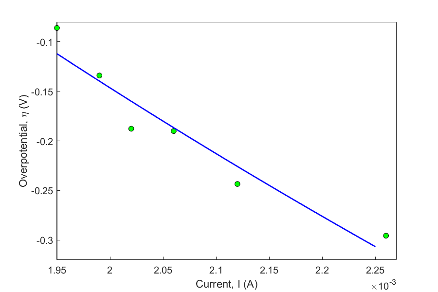
Figure 2 Overpotential as a function of current.\(\eta(V)\)
Power Functions
The power function equation describes many scientific and engineering phenomena. In chemical engineering, the rate of a chemical reaction is often written in power function form as
\[y = ax^{b} \;\;\;\;\;\;\;\;\;\;\;\; (11)\]
The least-squares method is applied to the power function by first transforming the data (the assumption is that \(b\) is not known). If the only unknown is \({ a}\), then a linear relation exists between \(x^{b}\) and\(\ y\).
When both \({a}\) and \({b}\) are unknowns, the transformation of the data is as follows.
\[\ln\left( y \right) = \ln\left( a \right) + b\ln\left( x \right)\;\;\;\;\;\;\;\;\;\;\;\; (12)\]
The resulting equation shows a linear relation between \(\ln y\) and \(\ln(x)\).
Let \[z = \ln y\]
\[w = \ln(x)\]
\[a_{0} = \ln a\ \text{implying}\ a = e^{a_{0}}\]
\[a_{1} = b\]
we get
\[z = a_{0} + a_{1}w\]
\[{a_{1} = \frac{\displaystyle n\sum_{i = 1}^{n}{w_{i}z_{i} - \displaystyle \sum_{i = 1}^{n}w_{i}}\displaystyle \sum_{i = 1}^{n}z_{i}}{n\displaystyle \sum_{i = 1}^{n}{w_{i}^{2} - \left(\displaystyle \sum_{i = 1}^{n}w_{i} \right)^{2}}} }\]
\[{a_{0} = \frac{\displaystyle \sum_{i = 1}^{n}z_{i}}{n} - a_{1}\frac{\displaystyle \sum_{i = 1}^{n}w_{i}}{n} }\;\;\;\;\;\;\;\;\;\;\;\; (13)\]
Since \(a_{0}\) and \(a_{1}\) can be found, the original constants of the model are
\[\begin{split} b &= a_{1}\\ a &= e^{a_{0}}\;\;\;\;\;\;\;\;\;\;\;\; (14a,b) \end{split}\]
Example 3
The progress of a homogeneous chemical reaction is followed, and it is desired to evaluate the rate constant and the order of the reaction. The rate law expression for the reaction is known to follow the power function form
\[- r = kC^{n}\]
Use the data provided in the table to obtain \(n\) and \(k\).
Table 4 Chemical kinetics.
| \(C_A(\text{gmol/l})\) | \(4\) | \(2.25\) | \(1.45\) | \(1.0\) | \(0.65\) | \(0.25\) | \(0.006\) |
|---|---|---|---|---|---|---|---|
| \(-r_A(\text{gmol/l}\cdot \text{s})\) | \(0.398\) | \(0.298\) | \(0.238\) | \(0.198\) | \(0.158\) | \(0.098\) | \(0.048\) |
Solution
Taking the natural log of both sides of Equation (35), we obtain
\[\ln\left( - r \right) = \ln\left( k \right) + n\ln\left( C \right)\;\;\;\;\;\;\;\;\;\;\;\; (E3.1)\]
Let
\[z = \ln\left( - r \right)\]
\[w = \ln\left( C \right)\]
\[a_{0} = \ln(k)\] implying that
\[\begin{split} k &= e^{a_{0}}\\ a_{1} &= n\;\;\;\;\;\;\;\;\;\;\;\; (3.2a,b)\end{split}\]
We get
\[z = a_{0} + a_{1}w\]
This is a linear relation between \(z\) and \(w\), where
\[a_{1} = \frac{m\displaystyle \sum_{i = 1}^{m}{w_{i}z_{i} - \sum_{i = 1}^{m}w_{i}}\sum_{i = 1}^{m}z_{i}}{m\displaystyle \sum_{i = 1}^{m}{w_{i}^{2} - \left( \displaystyle \sum_{i = 1}^{m}w_{i} \right)^{2}}}\]
\[a_{0} = \frac{\displaystyle \sum_{i = 1}^{m}z_{i}}{m} - a_{1}\frac{\displaystyle \sum_{i = 1}^{m}w_{i}}{m}\;\;\;\;\;\;\;\;\;\;\;\; (E3.3)\]
Table 5 Kinetics rate law using power function
| \(i\) | \(C\) | \(-r\) | \(w\) | \(z\) | \(wz\) | \(w^2\) |
|---|---|---|---|---|---|---|
| \(1\) | \(4\) | \(0.398\) | \(1.3863\) | \(-0.92130\) | \(-1.2772\) | \(1.9218\) |
| \(2\) | \(2.25\) | \(0.298\) | \(0.8109\) | \(-1.2107\) | \(-0.9818\) | \(0.65761\) |
| \(3\) | \(1.45\) | \(0.238\) | \(0.3716\) | \(-1.4355\) | \(-0.5334\) | \(0.13806\) |
| \(4\) | \(1\) | \(0.198\) | \(0.0000\) | \(-1.6195\) | \(0.0000\) | \(0.00000\) |
| \(5\) | \(0.65\) | \(0.158\) | \(-0.4308\) | \(-1.8452\) | \(0.7949\) | \(0.18557\) |
| \(6\) | \(0.25\) | \(0.098\) | \(-1.3863\) | \(-2.3228\) | \(3.2201\) | \(1.9218\) |
| \(7\) | \(0.006\) | \(0.048\) | \(-5.1160\) | \(-3.0366\) | \(15.535\) | \(26.173\) |
| \(\displaystyle \sum_{i = 1}^{7}{}\) | \(-4.3643\) | \(-12.391\) | \(16.758\) | \(30.998\) |
\[m = 7\]
\[\sum_{i = 1}^{7}{w_{i} = - 4.3643}\]
\[\sum_{i = 1}^{7}{z_{i} = - 12.391}\]
\[\sum_{i = 1}^{7}{w_{i}z_{i} = 16.758}\]
\[\sum_{i = 1}^{7}{w_{i}^{2} = 30.998}\]
From Equation (E3.3)
\[\begin{split} a_{1} &= \frac{7 \times \left( 16.758 \right) - \left( - 4.3643 \right) \times \left( - 12.391 \right)}{7 \times \left( 30.998 \right) - \left( - 4.3643 \right)^{2}}\\ &= 0.31943 \end{split}\]
\[\begin{split} a_{0} &= \frac{- 12.391}{7} - \left( 0.31943 \right)\frac{- 4.3643}{7}\\ &= - 1.5711 \end{split}\]
From Equation (E3.2a) and (E3.2b), we obtain
\[k = e^{- 1.5711} = 0.20782\]
\[n = a_{1} = 0.31941\]
Finally, the model of progress of that chemical reaction is
\[- r = 0.20782 \times C^{0.31941}\]
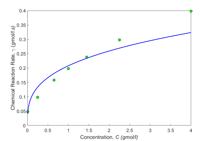
Figure 3 Kinetic chemical reaction rate as a function of concentration.
Multiple Choice Test
(1). When using transformed data to find the constants of the regression model \(y = ae^{{bx}}\) to best fit \(\left( x_{1},y_{1} \right),\left( x_{2},y_{2} \right),........\left( x_{n},y_{n} \right),\) the sum of the square of the residuals that is minimized is
(A) \(\displaystyle \sum_{i = 1}^{n}\left( y_{i} - {\ a}e^{bx_{i}} \right)^{2}\)
(B) \(\displaystyle \sum_{i = 1}^{n}\left( \ln(y_{i}) - \ln\left( a \right) - bx_{i} \right)^{2}\)
(C) \(\displaystyle \sum_{i = 1}^{n}\left( y_{i} - \ln\left( a \right) - bx_{i} \right)^{2}\)
(D) \(\displaystyle \sum_{i = 1}^{n}\left( \ln(y_{i}) - \ln\left( a \right) - b\ln(x_{i}) \right)^{2}\)
(2). It is suspected from theoretical considerations that the rate of water flow from a firehouse is proportional to some power of the nozzle pressure. Assume pressure data is more accurate. You are transforming the data.
| \(\text{Flow rate,}\ F\ (\text{gallons/min})\) | \(96\) | \(129\) | \(135\) | \(145\) | \(168\) | \(235\) |
|---|---|---|---|---|---|---|
| \(\text{Pressure},\ p\ (\text{psi})\) | \(11\) | \(17\) | \(20\) | \(25\) | \(40\) | \(55\) |
The exponent of the nozzle pressure in the regression model \(F = ap^{b}\) most nearly is
(A) \(0.49721\)
(B) \(0.55625\)
(C) \(0.57821\)
(D) \(0.67876\)
(3). The stress-strain curve is given as \(\sigma = k_{1}\varepsilon e^{- k_{2}\varepsilon}\) for concrete in compression, where \(\sigma\) is the stress and \(\varepsilon\) is the strain. To transform the data, one would use the following form
(A) \(\ln\left( \sigma \right) = \ln\left( k_{1} \right) + \ln\left( \varepsilon \right) - k_{2}\varepsilon\)
(B) \(\ln\left( \displaystyle \frac{\sigma}{\varepsilon} \right) = \ln\left( k_{1} \right) - k_{2}\varepsilon\)
(C) \(\ln\left( \displaystyle \frac{\sigma}{\varepsilon} \right) = \ln\left( k_{1} \right) + k_{2}\varepsilon\)
(D) \(\ln\left( \sigma \right) = \ln(k_{1}\varepsilon) - k_{2}\varepsilon\)
(4). In nonlinear regression, finding the constants of the model requires solving simultaneous nonlinear equations. However, in the exponential model \(y = ae^{{bx}}\) that is best fit to \(\left( x_{1},y_{1} \right),\left( x_{2},y_{2} \right),........,\left( x_{n},y_{n} \right),\) the value of \(b\) can be found as a solution of a single nonlinear equation. That nonlinear equation is given by
(A) \(\displaystyle \sum_{i = 1}^{n}{y_{i}x_{i}e^{bx_{i}} - \sum_{i = 1}^{n}{y_{i}e^{bx_{i}}\sum_{i = 1}^{n}x_{i} = 0}}\)
(B) \(\displaystyle \sum_{i = 1}^{n}{y_{i}x_{i}e^{bx_{i}}} - \frac{\displaystyle \sum_{i = 1}^{n}{y_{i}e^{bx_{i}}}}{\displaystyle\sum_{i = 1}^{n}e^{2bx_{i}}}\sum_{i = 1}^{n}{x_{i}e^{2bx_{i}}} = 0\)
(C) \(\displaystyle \sum_{i = 1}^{n}{y_{i}x_{i}e^{bx_{i}}} - \frac{\displaystyle\sum_{i = 1}^{n}{y_{i}e^{bx_{i}}}}{\displaystyle\sum_{i = 1}^{n}e^{2bx_{i}}}\sum_{i = 1}^{n}e^{bx_{i}} = 0\)
(D) \(\displaystyle \sum_{i = 1}^{n}{y_{i}e^{bx_{i}}} - \frac{\displaystyle\sum_{i = 1}^{n}{y_{i}e^{bx_{i}}}}{\displaystyle\sum_{i = 1}^{n}e^{2bx_{i}}}\sum_{i = 1}^{n}{x_{i}e^{2bx_{i}}} = 0\)
(5). There is a functional relationship between the mass density \(\rho\) of air and the altitude \(h\) above sea level.
| \(\text{Altitude above sea level},\ h\ (\text{km})\) | \(0.32\) | \(0.64\) | \(1.28\) | \(1.60\) |
|---|---|---|---|---|
| \(\text{Mass Density, }\rho\ (\text{kg/m}^3)\) | \(1.15\) | \(1.10\) | \(1.05\) | \(0.95\) |
In the regression model \(\rho = k_{1}e^{- k_{2}h}\), the constant \(k_{2}\) is found as \(k_{2} = 0.1315\). Assume the mass density of air at the top of the atmosphere is \(1/1000^{{th}}\) of the mass density of air at sea level. The altitude in kilometers of the top of the atmosphere most nearly is
(A) \(46.2\)
(B) \(46.6\)
(C) \(49.7\)
(D) \(52.5\)
(6). A steel cylinder at \(80{^\circ}\text{F}\) of length \(12^{\prime\prime}\) is placed in a commercially available liquid nitrogen bath\(( - 315{^\circ}\text{F})\). If the thermal expansion coefficient of steel behaves as a second-order polynomial function of temperature and the polynomial is found by regressing the data below,
| Temperature, \(T\ (^\circ\text{F})\) | Thermal expansion Coefficient, \(\alpha\) \((\mu \text{in/in/}^\circ \text{F})\) |
|---|---|
| \(- 320\) | \(2.76\) |
| \(- 240\) | \(3.83\) |
| \(- 160\) | \(4.72\) |
| \(- 80\) | \(5.43\) |
| \(0\) | \(6.00\) |
| \(80\) | \(6.47\) |
the reduction in the length of the cylinder in inches most nearly is
(A) \(0.0219\)
(B) \(0.0231\)
(C) \(0.0235\)
(D) \(0.0307\)
For complete solution, go to
http://nm.mathforcollege.com/mcquizzes/06reg/quiz_06reg_nonlinear_solution.pdf
Problem Set
(1). It is suspected from theoretical considerations that the rate of flow from a fire hose is proportional to some power of the nozzle pressure. Determine whether the speculation is true. What is the exponent of the data? Assume pressure data is more accurate. You are allowed to transform the data.
| \(\text{Flow rate}\ (\text{gallons/min}),\ F\) | \(94\) | \(118\) | \(147\) | \(180\) | \(230\) |
|---|---|---|---|---|---|
| \(\text{Pressure}\ (\text{psi}),\ p\) | \(10\) | \(16\) | \(25\) | \(40\) | \(60\) |
Answer: \(30.213 p^{0.49101}\)
(2). The following force vs. displacement data is given for a nonlinear spring.
| \(\text{Displacement},\ x\ (\text{m})\) | \(10\) | \(15\) | \(20\) |
|---|---|---|---|
| \(\text{Force},\ F\ (\text{N})\) | \(100\) | \(200\) | \(400\) |
Starting by minimizing the sum of the square of the residuals and without data transformation, the above \(F\) vs. \(x\) data is regressed to \(F = kx^{2}\). Find the value of \(k\).
Answer: \(0.97450\ \text{N/m}^2\)
(3). Data points \((x_{1},y_{1}),(x_{2},y_{2}),......,(x_{n},y_{n})\) is regressed to \(y = \displaystyle \frac{1}{(ax + b)^{2}}\). The constants of the model, \(a\) and \(b\) are solved by data transformation. Find the formulas for calculating \(a\) and \(b\)?
Hint: Take the inverse and square-root of both sides to transform the data
Answer: Answer not shown intentionally - follow the hint.
(4). Fit the regression model \(\sigma = K_{1}\varepsilon e^{\displaystyle {- K_{2}\varepsilon}}\) to the following stress-strain data of concrete. You are allowed to transform the data. Units of stress, \(\sigma\) are \(\text{psi},\) and units of strain, \(\varepsilon\) are \(\mu\text{in/in}\).
| \(\text{Stress},\ \sigma\ (\text{psi})\) | \(2250\) | \(3575\) | \(4250\) | \(4400\) | \(4200\) |
|---|---|---|---|---|---|
| \(\text{Strain,}\ \varepsilon\ (\mu\text{in/in})\) | \(500\) | \(1000\) | \(1500\) | \(2000\) | \(2375\) |
Answer: \(K_1=5.8406\), \(K_2= 4.9439\times10^{-4}\) (note the units for strain for which this \(K_2\) is given is \(\mu \text{in/in}\)). In the final answer, strain is in \(\mu \text{in/in}\), and stress in \(\text{psi}\). The units of \(K_2\) are \(\text{in}/ \mu \text{in}\). The units of \(K_1\) are \(\text{psi}/( \mu \text{in/in})\) which is the same as \(\text{Msi}\).
(5). It is desired to obtain a functional relationship between the mass density \(\rho\) of air and the altitude \(h\) above the sea level for the dynamic analysis of bodies moving within the earth’s atmosphere. Use the regression model \(\rho = k_{1}e^{- k_{2}h}\) to fit the data given below. Find the constants \(k_{1}\) and \(k_{2}\). You are allowed to transform the data.
Altitude (kilometers) |
Mass density (kg/m3) |
|---|---|
\(0.32\) \(0.64\) \(1.28\) \(1.60\) |
\(1.15\) \(1.10\) \(1.05\) \(0.95\) |
Answer: \(k_1=1.2053,\ k_2= 0.13395\), where in the model, \(h\) is in \(\text{kms}\), and \(\rho\) is in \(\text{kg/m}^3\)
(6). You are working for Valdez SpillProof Oil Company as a petroleum engineer. Your boss is asking you to estimate the life of an oil well. The analysis used in the industry is called the decline curve analysis, where the barrels of oil produced per unit time are plotted against time, and the curve is extrapolated. One of the standard curves used is the harmonic decline model, that is
\[q = \frac{b}{1 + at}\]
where \(q\) is the rate of production and \(t\) is the time, \(b\) and \(a\) are the constants of the regression model.
| \(\text{Time}\ (t),\ \text{month}\) | \(2\) | \(6\) | \(10\) | \(14\) | \(18\) |
|---|---|---|---|---|---|
| \(\text{Rate of production}\ (q),\ \text{barrels per day}\) | \(260\) | \(189\) | \(120\) | \(87\) | \(75\) |
a) Find the constants of the regression model. Hint: You are allowed to transform the data, if possible.
b) Find the total life of an oil field if \(5\) barrels per day is considered the production at which the field needs to be abandoned for further production.
c) What does \(b\) stand for physically?
Answer: \(a)\ 461.85/(1+0.29069t)\)
\(b)\ 314.30\ \text{months}\)
\(c) \text{Answer not given intentionally}\)
(7). From the physical understanding of a phenomenon, the velocity of a body is suspected to follow the relationship \(v = at^{2}\), where \(v\) is the velocity and \(t\) is the time. Given \(n\) data points \((t_{1},v_{1}),(t_{2},v_{2}),......,(t_{n},v_{n})\), start from the fundamentals of minimizing the sum of the squares of the residuals to derive a single equation in terms of the time and velocity data to find the value of \(a\). Simplify the equation. Show fill derivation that includes that the derived value of \(a\) corresponds to an absolute minimum of the sum of the squares of the residuals. You are not allowed to transform the data.
Answer: \(a=\displaystyle \frac{\displaystyle\sum^n_{i=1}v_it_i^2}{\displaystyle\sum^n_{i=1}t_i^4}\)
(8). The population for a small community is given as a function of time.
| \(\text{time, }t\ (\text{years})\) | \(0\) | \(5\) | \(10\) |
|---|---|---|---|
| \(\text{Population},\ p\) | \(100\) | \(165\) | \(314\) |
By minimizing the sum of the square of the residuals and without data transformation, the model is regressed to \(p = ae^{{bt}}\), where \(a\) and \(b\) are constants of the model. The value of \(b\) was found to be \(0.1199\). Find the value of \(a\).
Answer: \(p=94.136e^{0.1199t}\)
(9). The data given above is actually the weight (lbs) of a baby as a function of the age (months) of the baby
| \(t\) | \(0\) | \(2\) | \(4\) | \(6\) | \(18\) |
|---|---|---|---|---|---|
| \(W\) | \(7.5\) | \(11.25\) | \(14.30\) | \(16.00\) | \(26.00\) |
a) Fit \(W = at^{2} + bt + c\) to the data to find \(W(360)\)
b) We expect that the weight of the baby to saturate as the baby reaches adulthood. Suggest a different model and estimate \(W(360)\). Compare your results with part(a).
Answer: \(a)\ W=-0.03642t^2+1.6659t+7.7810;\ W(360)=-4110.2\)
\(b)\ \text{Answer intentionally not given}\)
(10). The temperature of a copper sphere cooling in air is measured as a function of time to yield the following data.
| \(\text{Time,}\ t\ (\text{s})\) | \(0.2\) | \(0.6\) | \(1.0\) | \(2.0\) |
|---|---|---|---|---|
| \(\text{Temperature},\ T\ (\text{C})\) | \(146.0\) | \(129.5\) | \(114.8\) | \(85.1\) |
From theoretical considerations, an exponential decrease of temperature is expected as a function of time. One can assume a regression model given by \(T = Ae^{- 0.3t}\) . Starting from minimizing the sum of the squares of the residuals, find the constant of the model, \(A\).
Answer: \(A=155.02\)
(11). There is a functional relationship between the mass density \(\rho\) of air and altitude \(h\) above sea level, and this is found from the data below.
| \(\text{Altitude above sea level},\ h\ (\text{km})\) | \(0.32\) | \(0.64\) | \(1.28\) | \(1.60\) |
|---|---|---|---|---|
| \(\text{Mass Density},\ \rho\ (\text{kg/m}^3)\) | \(1.15\) | \(1.10\) | \(1.05\) | \(0.95\) |
This functional relationship is found by regression using the model \(\rho = k_{1}e^{- k_{2}h}\). The constant \(k_{2}\) is found as \(k_{2} = 0.1315\). Assuming the mass density of air at the top of the atmosphere is \(1/1000^{{th}}\) of the mass density of air at sea level, find the altitude above the sea level in kilometers of the top of the atmosphere.
Answer: \(52.53\ \text{km}\)