Chapter 04.00: Physical Problem for Simultaneous Linear Equations
Summary
To find the velocity profile of a rocket requires a solution of simultaneous linear equations.
Modeling
The upward velocity of a rocket is given at three different times in the following table
| Time, t | Velocity, v |
|---|---|
| \(\text{s}\) | \(\text{m/s}\) |
| \(5\) | \(106.8\) |
| \(8\) | \(177.2\) |
| \(12\) | \(279.2\) |
The velocity data is approximated by a polynomial as
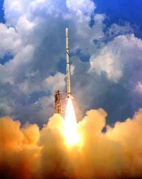
Figure 1 A rocket launched into space
\[v\left( t \right) = at^{2} + bt + c, \ 5 \leq t \leq 12.\;\;\;\;\;\;\;\;\;\;\;\; (1)\]
Set up the equations in matrix form to find the coefficients \(a,\ b,\ c\) of the velocity profile.
The polynomial is going through three data points \(\left( t_{1},v_{1} \right),\left( t_{2},v_{2} \right)\text{, and }\left( t_{3},v_{3} \right)\) where from the above table
\[t_{1} = 5,v_{1} = 106.8\]
\[t_{2} = 8,v_{2} = 177.2\]
\[t_{3} = 12,v_{3} = 279.2\]
Requiring that \(v\left( t \right) = at^{2} + bt + c\) passes through the three data points gives
\[\begin{split} v\left( t_{1} \right) &= v_{1} = at_{1}^{2} + bt_{1} + c\\ v\left( t_{2} \right) &= v_{2} = at_{2}^{2} + bt_{2} + c\\ v\left( t_{3} \right) &= v_{3} = at_{3}^{2} + bt_{3} + c \end{split}\]
Substituting the data \(\left( t_{1},\ v_{1} \right),\ \left( t_{2},\ v_{2} \right),\ \left( t_{3},\ v_{3} \right)\) gives
\[\begin{split} a\left( 5^{2} \right) + b\left( 5 \right) + c &= 106.8\\ a\left( 8^{2} \right) + b\left( 8 \right) + c &= 177.2\\ a\left( 12^{2} \right) + b\left( 12 \right) + c &= 279.2 \end{split}\]
or
\[\begin{split} 25a + 5b + c &= 106.8\\ 64a + 8b + c &= 177.2\\ 144a + 12b + c &= 279.2 \end{split}\]
This set of equations can be rewritten in the matrix form as
\[\begin{bmatrix} 25a + & 5b + & c \\ 64a + & 8b + & c \\ 144a + & 12b + & c \\ \end{bmatrix} = \begin{bmatrix} 106.8 \\ 177.2 \\ 279.2 \\ \end{bmatrix}\]
The above equation can be written as a linear combination as follows
\[a\begin{bmatrix} 25 \\ 64 \\ 144 \\ \end{bmatrix} + b\begin{bmatrix} 5 \\ 8 \\ 12 \\ \end{bmatrix} + c\begin{bmatrix} 1 \\ 1 \\ 1 \\ \end{bmatrix} = \begin{bmatrix} 106.8 \\ 177.2 \\ 279.2 \\ \end{bmatrix}\]
and further using matrix multiplications gives
\[\begin{bmatrix} 25 & 5 & 1 \\ 64 & 8 & 1 \\ 144 & 12 & 1 \\ \end{bmatrix}\ \begin{bmatrix} a \\ b \\ c \\ \end{bmatrix} = \begin{bmatrix} 106.8 \\ 177.2 \\ 279.2 \\ \end{bmatrix}\]
The solution of the above three simultaneous linear equations will give the value of \(a,b,c\).
Questions
(1) Solve for the values of \(a,b,c\).
(2) Verify if you get back the value of the velocity data at \(t=5\ \text{s}\).
(3) Estimate the velocity of the rocket at \(t=7.5\ \text{s}\)?
(4) Estimate the acceleration of the rocket at \(t=7.5\ \text{s}\)?
(5) Estimate the distance covered by the rocket between \(t=5.5\ \text{s}\) and \(8.9\ \text{s}\).
(6) If the following data is given for the velocity of the rocket as a function of time, and you are asked to use a quadratic polynomial to approximate the velocity profile to find the velocity at \(t=16\ \text{s}\), what data points would you choose and why?
| t | v(t) |
|---|---|
| \(\text{s}\) | \(\text{m/s}\) |
| \(0\) | \(0\) |
| \(10\) | \(227.04\) |
| \(15\) | \(362.78\) |
| \(20\) | \(517.35\) |
| \(22.5\) | \(602.97\) |
| \(30\) | \(901.67\) |
Modeling
Liquid-liquid extraction depends on the ability of some metal ions to form metal complexes with organic acids. The method is used to separate, concentrate, and purify metals and organic compounds. Liquid-liquid extraction was the technique used to produce weapon grade uranium during the arms race (cold war) era. The technique is also used to recover noble metals used in catalytic processes such as oil refining etc.
In liquid-liquid extraction, the metal ion in the aqueous phase is recovered by mixing the aqueous phase with an organic phase. The metal ion forms a complex with the organic phase and floats on top of the aqueous phase. The organic phase can be decanted and separated from the aqueous phase and the complexed metal ion recovered in a useful form using an acid (nitric acid for nitrates, sulfuric acid for sulfates etc).
A liquid-liquid extraction process conducted in the Electrochemical Materials Laboratory involved the extraction of nickel from the aqueous phase into an organic phase. A typical experimental data from the laboratory is given in Table 1.
Table 1 Aqueous and organic phase concentration of nickel.
| Ni aqueous phase (g/l) | \(2\) | \(2.5\) | \(3\) | \(3.5\) | \(4\) |
|---|---|---|---|---|---|
| Ni organic phase (g/l) | \(8.57\) | \(10\) | \(12\) | \(14\) | \(15.66\) |
Estimate the amount of nickel in organic phase when 2.3 g/l is in the aqueous phase. Use quadratic interpolation.
The polynomial is going through three data points \[\left( a_{1},g_{1} \right),\ \left( a_{2},g_{2} \right)\text{, and}\left( a_{3},g_{3} \right)\] where from the above table
\[a_{1} = 2,g_{1} = 8.57\]
\[a_{2} = 2.5,g_{2} = 10\]
\[a_{3} = 3,g_{3} = 12\]
Requiring that \(g = x_{1}a^{2} + x_{2}a + x_{3}\) passes through the three data points gives
\[g\left( a_{1} \right) = g_{1} = x_{1}a_{1}^{2} + x_{2}a_{1} + x_{3}\]
\[g\left( a_{2} \right) = g_{2} = x_{1}a_{2}^{2} + x_{2}a_{2} + x_{3}\]
\[g\left( a_{3} \right) = g_{3} = x_{1}a_{3}^{2} + x_{2}a_{3} + x_{3}\]
Substituting the data
\[\left( a_{1},g_{1} \right),\ \left( a_{2},{\ }{g}_{2} \right),\ \left( a_{3},{\ }{g}_{3} \right)\]
\[x_{1}\left( 2 \right)^{2} + x_{2}\left( 2 \right) + x_{3} = 8.57\]
\[x_{1}\left( 2.5 \right)^{2} + x_{2}\left( 2.5 \right) + x_{3} = 10\]
\[x_{1}\left( 3 \right)^{2} + x_{2}\left( 3 \right) + x_{3} = 12\]
gives
\[4x_{1} + 2x_{2} + x_{3} = 8.57\]
\[6.25x_{1} + 2.5x_{2} + x_{3} = 10\]
\[9x_{1} + 3x_{2} + x_{3} = 12\]
This set of equations can be rewritten in the matrix form as
\[\begin{bmatrix} 4x_{1} + & 2x_{2} + & x_{3} \\ 6.25x_{1} + & 2.5x_{2} + & x_{3} \\ 9x_{1} + & 3x_{2} + & x_{3} \\ \end{bmatrix} = \begin{bmatrix} 8.57 \\ 10 \\ 12 \\ \end{bmatrix}\]
The above equations can be written as a linear combination as follows
\[x_{1}\begin{bmatrix}4 \\ 6.25 \\ 9 \\ \end{bmatrix} + x_{2}\begin{bmatrix} 2 \\ 2.5 \\ 3 \\ \end{bmatrix} + x_{3}\begin{bmatrix} 1 \\ 1 \\ 1 \\ \end{bmatrix} = \begin{bmatrix} 8.57 \\ 10 \\ 12 \\ \end{bmatrix}\]
and further using matrix multiplication gives
\[\begin{bmatrix} 4 & 2 & 1 \\ 6.25 & 25 & 1 \\ 9 & 3 & 1 \\ \end{bmatrix}\ \begin{bmatrix} x_{1} \\ x_{2} \\ x_{3} \\ \end{bmatrix} = \begin{bmatrix} 8.57 \\ 10 \\ 12 \\ \end{bmatrix}\]
The solution of the above simultaneous linear equations will give the value of \(x_{1},x_{2},x_{3}.\)
Questions
(1) Verify if you get back the value of the Ni organic phase when the Ni aqueous phase is 2.5 g/l.
(2) Estimate the value of the Ni organic phase when the Ni aqueous phase is 2.78 g/l
(3) Estimate the error between linear interpolation and quadratic interpolation values obtained for nickel in organic phase when 2.78 g/l is in the aqueous phase.
Summary
A pressure vessel made of a compounded cylinder has a higher capability to handle internal pressure over a single cylinder. To find this capability, one has to solve a set of simultaneous linear equations.
Modeling
A pressure vessel can only be subjected to an amount of internal pressure that is limited by the strength of the material used. For example, take a pressure vessel of an internal radius of \(a = 5^{\prime\prime}\) and outer radius, \(b = 8^{\prime\prime}\), made of ASTM 36 steel (yield strength of ASTM 36 steel is 36 ksi). How much internal pressure can this pressure vessel take before it is considered to have failed?
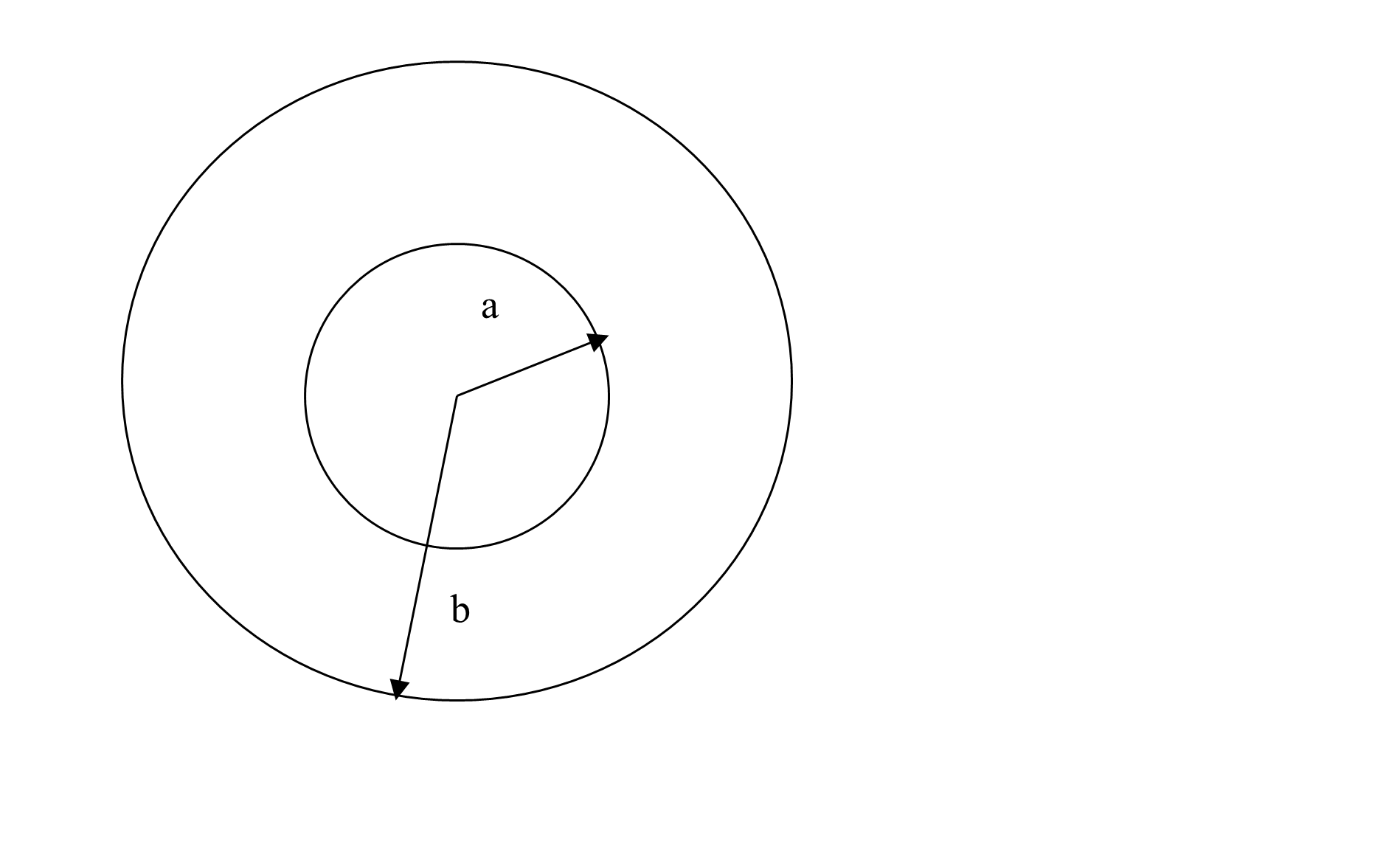
Figure 1 A single-cylinder pressure vessel with internal radius, \(a\) and outer radius, \(b\).
The hoop and radial stress in a cylindrical pressure vessel is given by [1]
\[\sigma_{r} = \frac{a^{2}p_{i}}{b^{2} - a^{2}}\left( 1 - \frac{b^{2}}{r^{2}} \right)\;\;\;\;\;\;\;\;\;\;\;\; (1)\]
\[\sigma_{\theta} = \frac{a^{2}p_{i}}{b^{2} - a^{2}}\left( 1 + \frac{b^{2}}{r^{2}} \right)\;\;\;\;\;\;\;\;\;\;\;\; (2)\]
The maximum normal stress anywhere in the cylinder is the hoop stress at the inner radius, \(a\)
\[{\left. \ \sigma_{\theta} \right|i\left( \frac{b^{2} + a^{2}}{b^{2} - a^{2}} \right)}_{\max}\;\;\;\;\;\;\;\;\;\;\;\; (3)\]
Assuming a factor of safety of 2, while the yield strength is given as 36 ksi,
\[\frac{36 \times 10^{3}}{2} = p_{i}\left( \frac{8^{2} + 5^{2}}{8^{2} - 5^{2}} \right)\]
\[p_{i} = 7.887{ksi}\]
You can see from Equation (3) that even for \(b > > a\), the maximum internal pressure one can apply is only \(p_{i} = 18{ksi}\). Therefore, what can an engineer do to maximize the internal pressure while keeping the material and radial dimensions the same? They can use a compounded cylinder. They can create a compounded cylinder by shrink fitting one cylinder into another, and hence creating pre-existing favorable stresses to allow more internal pressure. Let us see how that would work?
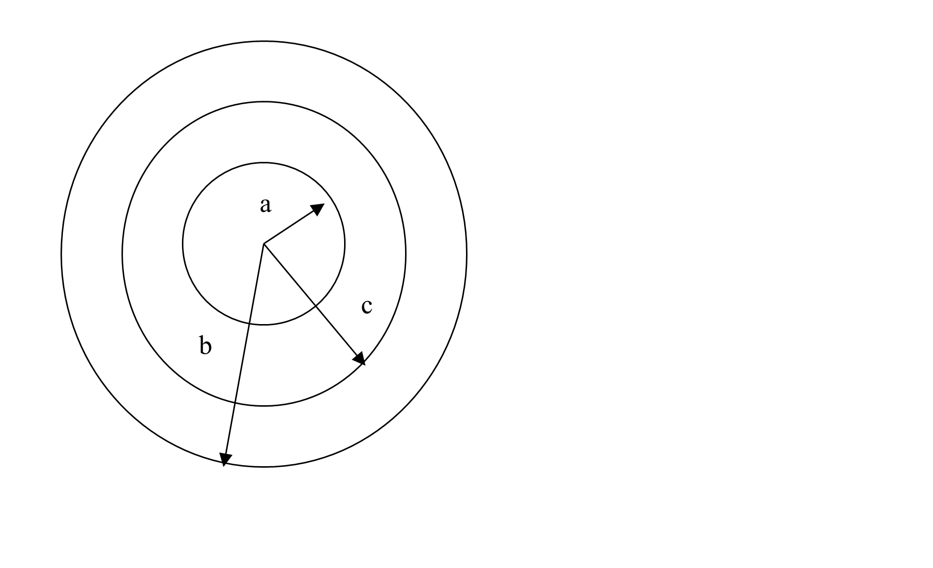
Figure 2 A compounded cylinder pressure vessel with internal radius, \(a\), outer radius, \(b\), and interface at \(r = c\).
Let us make the compounded cylinder of two cylinders (Figure 2). Cylinder 1 has an internal radius of \(a = 5^{\prime\prime}\), and outer radius \(c = 6.5^{\prime\prime}\), while Cylinder 2 has an internal radius of \(c = 6.5^{\prime\prime}\) and outer radius, \(b = 8^{\prime\prime}\). Assume that that radial interference, \(\delta = 0.007^{\prime\prime}\) occurs at the interface of a compounded cylinder at \(r = c = 6.5^{\prime\prime}\). How does then one find the pressure that can be applied to the compounded cylinder of internal radius, \(a = 5^{\prime\prime}\) and outer radius, \(b = 8^{\prime\prime}\)?
For cylinder 1, the radial displacement, \(u_{1}\) is given by
\[u_{1} = c_{1}r + \frac{c_{2}}{r}\;\;\;\;\;\;\;\;\;\;\;\; (4)\]
the radial stress, \(\sigma_{r}^{1}\)and hoop stress, \(\sigma_{\theta}^{1}\) by
\[\sigma_{r}^{1} = \frac{E}{1 - \nu^{2}}\left\lbrack c_{1}\left( 1 + \nu \right) - c_{2}\left( \frac{1 - \nu}{r^{2}} \right) \right\rbrack\;\;\;\;\;\;\;\;\;\;\;\; (5)\]
\[\sigma_{\theta}^{1} = \frac{E}{1 - \nu^{2}}\left\lbrack c_{1}\left( 1 + \nu \right) + c_{2}\left( \frac{1 - \nu}{r^{2}} \right) \right\rbrack\;\;\;\;\;\;\;\;\;\;\;\; (6)\]
where
\[E = \text{Young's modulus of steel,}\]
\[\nu = \text{Poisson's ratio of steel.}\]
For cylinder 2, the radial displacements, \(u_{2}\)is given by
\[u_{2} = c_{3}r + \frac{c_{4}}{r}\;\;\;\;\;\;\;\;\;\;\;\; (7)\]
the radial stress, \(\sigma_{r}^{2}\) and hoop stress, \(\sigma_{\theta}^{2}\) by
\[\sigma_{r}^{2} = \frac{E}{1 - \nu^{2}}\left\lbrack c_{3}\left( 1 + \nu \right) - c_{4}\left( \frac{1 - \nu}{r^{2}} \right) \right\rbrack\;\;\;\;\;\;\;\;\;\;\;\; (8)\]
\[\sigma_{\theta}^{2} = \frac{E}{1 - \nu^{2}}\left\lbrack c_{3}\left( 1 + \nu \right) + c_{4}\left( \frac{1 - \nu}{r^{2}} \right) \right\rbrack\;\;\;\;\;\;\;\;\;\;\;\; (9)\]
So if one is able to find the four constants, \(c_{1},c_{2},c_{3}\) and \(c_{4}\), one can find the stresses in the compounded cylinder to be able to find what internal pressure can be applied. So how do we find the four unknown constants?
The boundary and interface conditions are the following.
The radial stress at the inner radius, \(r = a\) is the applied internal pressure
\[\sigma_{r}^{1}\left( r = a \right) = - p_{i}\;\;\;\;\;\;\;\;\;\;\;\; (10)\]
The radial stress is continuous at the interface, \(r = c\)
\[\sigma_{r}^{1}\left( r = c \right) = \sigma_{r}^{2}\left( r = c \right)\;\;\;\;\;\;\;\;\;\;\;\; (11)\]
The radial displacement at the interface, \(r = c\) has a jump of the radial interference, \(\delta\)
\[u_{2}\left( r = c \right) - u_{1}\left( r = c \right) = \delta\;\;\;\;\;\;\;\;\;\;\;\; (12)\]
The radial stress at the outer radius, \(r = c\) is
\[\sigma_{r}^{2}\left( r = b \right) = 0\;\;\;\;\;\;\;\;\;\;\;\; (13)\]
This will set up four equations and four unknowns, if we know what internal pressure we are applying. Assume we are applying the same pressure as the single cylinder can take, that is,\(p_{i} = 7.887\)ksi and let us see later what stresses it creates in the compounded cylinder.
Assuming \(E = 30 \times 10^{6}\)psi, \(\nu = 0.3\), Equations (10) through (13) become
\[\frac{30 \times 10^{6}}{1 - 0.3^{2}}\left\lbrack c_{1}\left( 1 + 0.3 \right) - c_{2}\left( \frac{1 - 0.3}{5^{2}} \right) \right\rbrack = - 7.887 \times 10^{3}\]
\[\frac{30 \times 10^{6}}{1 - 0.3^{2}}\left\lbrack c_{1}\left( 1 + 0.3 \right) - c_{2}\left( \frac{1 - 0.3}{6.5^{2}} \right) \right\rbrack = \frac{30 \times 10^{6}}{1 - 0.3^{2}}\left\lbrack c_{3}\left( 1 + 0.3 \right) - c_{4}\left( \frac{1 - 0.3}{6.5^{2}} \right) \right\rbrack\]
\[c_{3}\left( 6.5 \right) + \frac{c_{4}}{6.5} - c_{1}\left( 6.5 \right) - \frac{c_{2}}{6.5} = 0.007\]
\[\frac{30 \times 10^{6}}{1 - 0.3^{2}}\left\lbrack c_{3}\left( 1 + 0.3 \right) - c_{4}\left( \frac{1 - 0.3}{8^{2}} \right) \right\rbrack = 0\;\;\;\;\;\;\;\;\;\;\;\; (14a-d)\]
Writing the Equations (14a-d) in matrix form, we get
\[\begin{bmatrix} 4.2857 \times 10^{7} & - 9.2307 \times 10^{5} & 0 & 0 \\ 4.2857 \times 10^{7} & - 5.4619 \times 10^{5} & - 4.2857 \times 10^{7} & 5.4619 \times 10^{5} \\ - 6.5 & - 0.15384 & 6.5 & 0.15384 \\ 0 & 0 & 4.2857 \times 10^{7} & - 3.6057 \times 10^{5} \\ \end{bmatrix}\begin{bmatrix} c_{1} \\ c_{2} \\ c_{3} \\ c_{4} \\ \end{bmatrix} = \begin{bmatrix} - 7.887 \times 10^{3} \\ 0 \\ 0.007 \\ 0 \\ \end{bmatrix}\;\;\;\;\;\;\;\;\;\;\;\; (15)\]
Solving these four simultaneous linear equations, we can find the four constants.
References
(1) A.C. Ugural, S.K. Fenster, Advanced strength and applied elasticity, Third Edition, Prentice Hall, New York, 1995.
(2) J.E. Shigley, C.R. Mischke, Chapter 19 - Limits and fits, Standard handbook of machine design, McGraw-Hill, New York, 1986.
Questions
(1) Find the unknown constants of Equation (14) using different numerical methods.
(2) Knowing that the critical points in the compounded cylinder are \(r = a,c - ,c + ,\text{and}\ b\), find the maximum hoop stress in the compounded cylinder. What is its value compared to the maximum hoop stress allowable of 18 ksi?
(3) Find the maximum internal pressure you can apply to the compounded cylinder? Compare it with the maximum possible internal pressure for a single cylinder of the same dimensions.
(4) The radial interference at the interface is created by making the inner cylinder 1 to have a larger outer radius than the inner radius of cylinder 2. Standard interference fits dictate the limits of these dimensions. If cylinder 2 is fit into cylinder 1, there is an upper and lower limit by which the nominal diameter of each cylinder varies at the interface. This limit L in thousands of an inch, is given by [2]
\[L = CD^{1/3}\] where \(D\) (nominal diameter) is in inches, and the coefficient \(C\),based on the type of fit, is given in Table 1 below.
| Cylinder | Limit | Class of fit | |
|---|---|---|---|
| FN2 | FN3 | ||
| \(1\) | \(\text{Lower}\) | \(0.000\) | \(0.000\) |
| \(\text{Upper}\) | \(0.907\) | \(0.907\) | |
| \(2\) | \(\text{Lower}\) | \(2.717\) | \(3.739\) |
| \(\text{Upper}\) | \(3.288\) | \(4.310\) |
Assuming FN2 fit at the interface, find the maximum internal pressure you would recommend.
Modeling
Human vision has the remarkable ability to infer 3D shapes from 2D images. When we look at 2D photographs or TV we do not see them as 2D shapes, rather as 3D entities with surfaces and volumes. Perception research has unraveled many of the cues that are used by us. The intriguing question is can we replicate some of these abilities on a computer? To this end, in this assignment we are going to look at one way to engineer a solution to the 3D shape from 2D images problem. Apart from the pure fun of solving a new problem, there are many practical applications of this technology such as in automated inspection of machine parts, inference of obstructing surfaces for robot navigation, and even in robot assisted surgery.
Image is a collection of gray level values at set of predetermined sites known as pixels, arranged in an array. These gray level values are also known as image intensities. The registered intensity at an image pixel is dependent on a number of factors such as the lighting conditions, surface orientation and surface material properties. The nature of lighting and its placement can drastically affect the appearance of a scene. Can we infer shape of the underlying surface given images as in the images below in Figure 1.
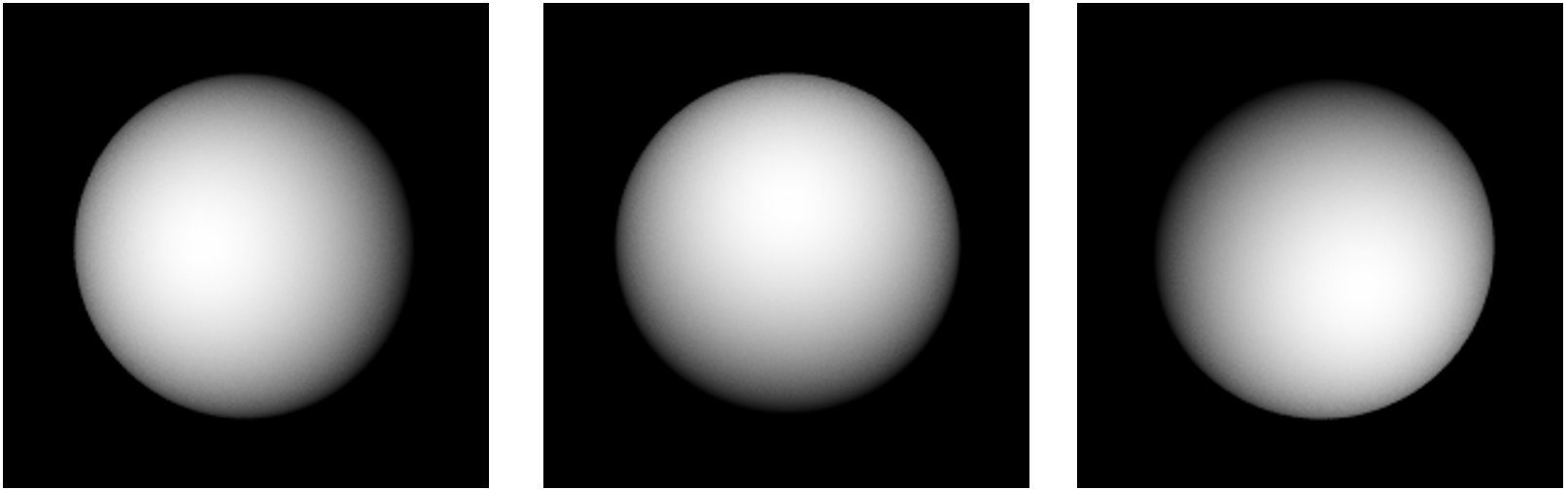
Figure 1 Images of a surface taken with three different light directions. Can you guess the shape of the underlying surface?
Physics of the Problem
To be able to reconstruct the shape of the underlying surface, we have to first understand the image formation process. The simplest image formation model assumes that the camera is far away from the scene so that we have assume that the image is a scaled version of the world. The simplest light model consists of a point light that is far away. This is not an unrealistic assumption. A good example of such a light source is the sun. We also assume that the surface is essentially matte that reflects lights uniformly in all directions, unlike specular (or mirror-like surfaces). These kinds of surfaces are called Lambertian surfaces; examples include walls, and carpet.
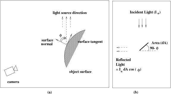
Figure 2 Relationship between the surface and the light source. (b) Amount of light reflected by an elemental area (dA) is proportional to the cosine of the angle between the light source direction and the surface normal
The image brightness of a Lambertian surface is dependent on the local surface orientation with respect to the light source. Since the point light source is far away we will assume that the incident light is locally uniform and comes from a single direction, i.e, the light rays are parallel to each other. This situation is illustrated in Figure 2. Let the incident light intensity be denoted by \(I_{0}\). Also let the angle between the light source and local surface orientation be denoted by \(\varphi\). Then the registered image intensity, \(I(u,v)\), of that point is given by
\[I(u,v) = I_{0}\rho\cos(\varphi) = I_{0}\rho(n_{x}s_{x} + n_{y}s_{y} + n_{z}s_{z})\]
where the surface normal, \(n\), and the light source direction, \(s\), are given by:
\[n^{\ } = \begin{bmatrix} n_{x} \\ n_{y} \\ n_{z} \\ \end{bmatrix},\ s = \begin{bmatrix} s_{x} \\ s_{y} \\ s_{z} \\ \end{bmatrix}\]
and \(\rho\) is a number capturing the surface reflection property at the location \((x,y)\), and It is referred to as the surface albedo. Black surfaces tend to have low albedo and white surfaces tend to high albedo. Note that the registered intensity in the image does not depend on the camera location because a Lambertian surface reflects light equally in all directions. This would not be true for specular surfaces and the corresponding image formation equation would involve the viewing direction.
The variation in image intensity is essentially dependent on the local surface orientation. If the surface normal and the light source directions are aligned then we have the maximum intensity and the observed intensity of the lowest when the angle between the light source and the local surface orientation is \(90^{0}\). Thus, given the knowledge of light source and the local surface albedo, it should be possible to infer the local surface orientation from the local image intensity variations. This is what we explore next.
The mapping of surface orientation to image intensity is many to one. Thus, it is not possible to infer the surface orientation from just one intensity image in the absence of any other knowledge. We need multiple samples per point in the scene. How many samples do we need? The vector specifying the surface normal has three components, which implies that we need three. So, we engineer a setup to infer surface orientation from image intensities. Instead of just one image of a scene, let us take three images of the same scene, without moving either the camera or the scene, but with three different light sources, turned on one at a time. These three different light sources are placed at different locations in space. Let the three light source directions, relative to the camera, be specified by the vectors
\[s^{1} = \begin{bmatrix} s_{x}^{1} \\ s_{y}^{1} \\ s_{z}^{1} \\ \end{bmatrix},\ s^{2} = \begin{bmatrix} s_{x}^{2} \\ s_{y}^{2} \\ s_{z}^{2} \\ \end{bmatrix},\ s^{3} = \begin{bmatrix} s_{x}^{3} \\ s_{y}^{3} \\ s_{z}^{3} \\ \end{bmatrix}\] Corresponding pixels in the three images would have three different intensities \(I_{1}\), \(I_{2}\), and \(I_{3}\) for three light source directions. Let the surface normal corresponding to the pixel under consideration be denoted by
\[n= \begin{bmatrix} n_{x} \\ n_{y} \\ n_{z} \\ \end{bmatrix}\]
Assuming Lambertian surfaces, the three intensities can be related to the surface normal and the light source directions
\[I_{i} = I_{0}\rho(n_{x}s_{x}^{i} + n_{y}s_{y}^{i} + n_{z}s_{z}^{i}),\ \forall i = 1,2,3\]
In these three equations, the known variables are the intensities, \(I_{1}\), \(I_{2}\), \(I_{3}\), and the light source directions, \(s_{1}\), \(s_{2}\), \(s_{3}\). The unknowns are the incident intensity, \(I_{3}\), surface albedo, \(\rho\) and the surface normal, \(n\). These unknowns can be bundled into three unknown variables, \(m_{x} = I_{0}\rho n_{x}\), \(m_{y} = I_{0}\rho n_{y}\), and \(m_{z} = I_{0}\rho n_{z}\). We will recover the surface normal by normalizing the recovered \(m\) vector, using the fact that the magnitude of the normal is one. The normalizing constant will give us the product \(I_{0}\rho\). Thus, for each point in the image, we have three simultaneous equations in three unknowns.
\[\begin{bmatrix} I_{1} \\ I_{2} \\ I_{3} \\ \end{bmatrix} = \begin{bmatrix} s_{x}^{1} & s_{y}^{1} & s_{z}^{1} \\ s_{x}^{2} & s_{y}^{2} & s_{z}^{2} \\ s_{x}^{3} & s_{y}^{3} & s_{z}^{3} \\ \end{bmatrix}\begin{bmatrix} m_{x} \\ m_{y} \\ m_{z} \\ \end{bmatrix}\]
Worked Out Example
Consider the middle of the sphere in Figure 1. We know that the surface normal points towards the camera (i.e. towards the viewer). Assume a 3D coordinate system centered at the camera with \(x\) -direction along the horizontal direction, \(y\) -direction along the vertical direction, and \(z\) -direction is away from the camera into the scene. Then the actual surface normal of the middle of the sphere is given by [0, 0, -1] – the negative denotes that it point in the direction opposite the z-axis. Let us see how close our estimate is to the actual value.
The intensity of the middle of the sphere in the three views, \(I_{1} = 247,\) \(I_{2} = 248,\) and \(I_{3} = 239\), respectively. The light directions for the three images are along [5, 0, -20], [0, 5, -20], and [-5, -5, -20], respectively. Normalizing the three vectors we get the normal directions towards the lights and construct the 3 by 3 matrix
\[\begin{bmatrix} s_{x}^{1} & s_{y}^{1} & s_{z}^{1} \\ s_{x}^{2} & s_{y}^{2} & s_{z}^{2} \\ s_{x}^{3} & s_{y}^{3} & s_{z}^{3} \\ \end{bmatrix} = \begin{bmatrix} 0.2425 & 0 & - 0.9701 \\ 0 & 0.2425 & - 0.9701 \\ - 0.2357 & - 0.2357 & - 0.9428 \\ \end{bmatrix}\]
Solving the corresponding 3 simultaneous equations, we arrive the following solution for the \(m\) -vector:
\[\begin{bmatrix} m_{x} \\ m_{y} \\ m_{z} \\ \end{bmatrix} = \begin{bmatrix} 0.0976 \\ 4.2207 \\ - 254.5774 \\ \end{bmatrix}\]
Normalizing this vector we get the surface normal
\[\begin{bmatrix} n_{x} \\ n_{y} \\ n_{z} \\ \end{bmatrix} = \begin{bmatrix} 0.0004 \\ 0.0166 \\ - 0.9999 \\ \end{bmatrix}\]
The corresponding normalizing constant is 254.6124, which is the product of the intensity of the illumination and the surface (albedo) reflectance factor \((I_{0}\rho)\). Compare the estimate of the surface normal to the actual one. The difference is quantization effects – in images we can represent intensities as a finite sized integer – 8-bit integers in our case.
We can repeat the above computations for each point in the scene to arrive at estimates of the corresponding surface normals. Figure 3(a) is a visualization of the surface normals thus estimated as a vector field. In Figure 3(b), we see the product \(I_{0}\rho\) visualized as image intensities. As expected, it is the same at all points on the sphere. In another problem module, how do we recover the underlying surface from these surface normals?
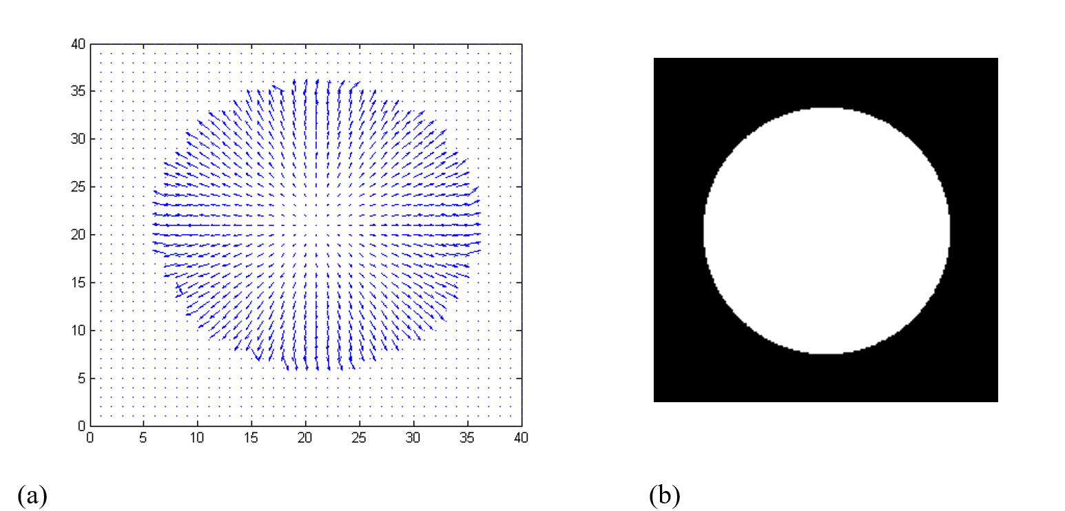
Figure 3 (a) Recovered surface normal at each point on the sphere. Just the first two components of the vectors are shown as a arrows. (b) Recovered product \(I_{0}\rho\) for all points
Questions
(1) What can you infer about the surface normal for the brightest point in the image? What about the darkest point in the scene?
(2) What assumptions do you have to make to make the above inferences?
Summary
Designing three-phase loads in AC systems require the solution of simultaneous linear equations.
Modeling
Three-phase AC systems are the norm for most industrial applications. AC power in the form of voltage and current it delivered from the power company using three-phase distribution systems and many larger loads are three-phase loads in the form of motors, compressors, or similar. Sources and loads can be configured in either wye (where sources or loads are connected from line to neutral/ground) or delta (where sources or loads are connected from line to line) configurations and mixing between the types is common. Figure 1 shows the general wiring of a wye-wye three-phase system modeling all of the impedances typically found in such a system.
During the typical analysis undertaken in most circuits textbooks, it is assumed that the system is entirely balanced. This means that all the source, line, and load impedances are equivalent, that is,
\[Z_{a} = Z_{b} = Z_{c}\]
\[Z_{{aA}} = Z_{{bB}} = Z_{{cC}}\]
\[Z_{{AN}} = Z_{{bN}} = Z_{{CN}}\]
Under this assumption, the circuit is then typically reduced to a single-phase equivalent circuit model and the resultant circuit is solved with a single loop equation. What happens, however, when the system is unbalanced? Typically because the three load impedances \(Z_{{AN}},Z_{{BN}}\) and \(Z_{{CN}}\) are not equal, which results in different currents through each load, is often measured in terms of the percentage difference between the load currents.
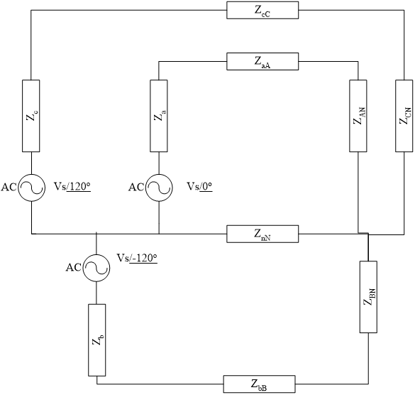
Figure 1 A Three-Phase Wye-Wye System with Positive Phase Sequence
Creating an imbalance in a three-phase system is not all that difficult. Consider a small business operating in an isolated leg of the power grid so that localized aspects of a load are not “balanced” by other neighboring loads. Let’s assume that the primary load for this system is a 45 kVA set of three-phase motors at 0.8 power factor lagging and, further, that the electrician that did the wiring for the lighting mistakenly connected two banks of lights to the A phase, one to the B phase and none to the C phase creating an imbalance in the system. Each of these lighting loads is 1500 W. The load for this system is shown in Figure 2.
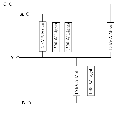
Figure 2 Model of the System Load
The impedance of each of the loads can be determined by examining the power consumed in each phase of the system
\[\begin{split} A:3000 + 15000/\underline{-36.87 ^{\circ}} &= 3000 + 12000 - j9000 = 15000 - j9000 \\ &= 17.49/\underline{-30.96^{\circ}} {kVA} \end{split}\]
\[\begin{split} B:1500 + 15000/\underline{-36.87^{\circ}} &= 1500 + 12000 - j9000 = 13500 - j9000 \\ &= 16.22/\underline{-33.69^{\circ}} {kVA} \end{split}\]
\[C:15.00/\underline{-36.87^{\circ}}{kVA}\]
Converting these to impedances using the formula \[S = \frac{\left| V \right|^{2}}{Z}\ \text{with}\ V = 120V \text{ yields}:\]
\[Z_{{AN}} = 0.8233/\underline{30.96^{\circ}}\Omega = R_{A} + jX_{A} = 0.7060 + j0.4236\Omega\]
\[Z_{{BN}} = 0.8878/\underline{33.39^{\circ}}\Omega = R_{B} + jX_{B} = 0.7387 + j0.4925\Omega\]
\[Z_{{CN}} = 0.9600/\underline{36.87^{\circ}}\Omega = R_{C} + jX_{C} = 0.7680 + j0.5760\Omega\]
For the rest of this analysis we will assume that each phase of the system has an equivalent source and line impedance of \(R_{s} + jX_{s} = 0.0300 + j0.0200\Omega\) and that the ground return wire has an impedance of\(R_{n} + jZ_{n} = 0.0100 + j0.0080\Omega\). This yields the equivalent circuit of Figure 3.
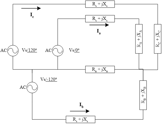
Figure 3 Equivalent Circuit Model for the Working Problem
The circuit can be analyzed using three loop equations using the currents \(I_{a},I_{b},\) and \(I_{c}\) shown in Figure 3. For loop A this yields the complex equation:
Loop A:
\[- V_{s}/\underline{0^{\circ}} + I_{a}\left( R_{s} + jX_{s} + R_{A} + jX_{A} \right) + \left( I_{a} + I_{b} + I_{c} \right)\left( R_{n} + jX_{n} \right) = 0\]
with loops B and C yielding similar results. Assuming that our simultaneous equation solver is not capable of handling complex numbers we can turn the loop A equation into two separate non-complex equations addressing both the real and imaginary parts. Using \(I_{a} = I_{{ar}} + jI_{{ai}}\) and collecting terms yields:
Real A:
\[I_{{ar}}\left( R_{s} + R_{A} + R_{n} \right) - I_{{ai}}\left( X_{s} + X_{A} + X_{n} \right) + I_{{br}}R_{n} - I_{{bi}}X_{n} + I_{{cr}}R_{n} - I_{{ci}}X_{n} = 120\ \ \ (1)\]
Imaginary A:
\[I_{{ar}}\left( X_{s} + X_{A} + X_{n} \right) + I_{{ai}}\left( R_{s} + R_{A} + R_{n} \right) + I_{{br}}X_{n} + I_{{bi}}R_{n} + I_{{cr}}X_{n} + I_{{ci}}R_{n} = 0\ \ \ (2)\]
Applying the same analysis to the B and C loops yields the remaining equations for the system.
Real B:
\[I_{{ar}}R_{n} - I_{{ai}}X_{n} + I_{{br}}\left( R_{s} + R_{B} + R_{n} \right) - I_{{bi}}\left( X_{s} + X_{B} + X_{n} \right) + I_{{cr}}R_{n} - I_{{ci}}X_{n} = - 60\ \ \ (3)\]
Imaginary B:
\[I_{{ar}}X_{n} + I_{{ai}}R_{n} + I_{{br}}\left( X_{s} + X_{B} + X_{n} \right) + I_{{bi}}\left( R_{s} + R_{B} + R_{n} \right) + I_{{cr}}X_{n} + I_{{ci}}R_{n} = - 103.9\ \ \ (4)\]
Real C:
\[I_{{ar}}R_{n} - I_{{ai}}X_{n} + I_{{br}}R_{n} - I_{{bi}}X_{n} + I_{{cr}}\left( R_{s} + R_{C} + R_{n} \right) - I_{{ci}}\left( X_{s} + X_{C} + X_{n} \right) = - 60\ \ \ (5)\]
Imaginary C:
\[I_{{ar}}X_{n} + I_{{ai}}R_{n} + I_{{br}}X_{n} + I_{{bi}}R_{n} + I_{{cr}}\left( X_{s} + X_{C} + X_{n} \right) + I_{{ci}}\left( R_{s} + R_{C} + R_{n} \right) = 103.9\ \ \ (6)\]
This yields a system of six linear equations and six unknowns \(\left( I_{{ar}},I_{{ai}},I_{{br}},I_{{bi}},I_{{cr}},{\ and\ }I_{{ci}} \right)\) that can be solved by any conventional means. This is shown in matrix form in Figure 4.
\[\begin{bmatrix} 0.7460 & - 0.4516 & 0.0100 & - 0.0080 & 0.0100 & - 0.0080 \\ 0.4516 & 0.7460 & 0.0080 & 0.0100 & 0.0080 & 0.0100 \\ 0.0100 & - 0.0080 & 0.7787 & - 0.5205 & 0.0100 & - 0.0080 \\ 0.0080 & 0.0100 & 0.5205 & 0.7787 & 0.0080 & 0.0100 \\ 0.0100 & - 0.0080 & 0.0100 & - 0.0080 & 0.8080 & - 0.6040 \\ 0.0080 & 0.0100 & 0.0080 & 0.0100 & 0.6040 & 0.8080 \\ \end{bmatrix}\begin{bmatrix} I_{{ar}} \\ I_{{ai}} \\ I_{{br}} \\ I_{{bi}} \\ I_{{cr}} \\ I_{{ci}} \\ \end{bmatrix} = \begin{bmatrix} 120.0 \\ 0.000 \\ - 60.00 \\ - 103.9 \\ - 60.00 \\ 103.9 \\ \end{bmatrix}\ \ \ (7)\]
Figure 4 Complete System of Equations
Once the currents are known it is a simple procedure to determine the voltages across the three motor terminals \(\left( V_{{AN}},V_{{BN}},{\ and\ }V_{{CN}} \right)\) using Ohm’s Law.
\[V_{{AN}} = \left( I_{{ar}} + jI_{{ai}} \right)\left( R_{A} + jX_{A} \right)\]
\[V_{{BN}} = \left( I_{{br}} + jI_{{bi}} \right)\left( R_{B} + jX_{B} \right)\]
\[V_{{CN}} = \left( I_{{cr}} + jI_{{ci}} \right)\left( R_{C} + jX_{C} \right)\]
To better evaluate the imbalance, the percentage difference in currents through the actual load elements is more often considered. The best way to think of this as three people pulling and pushing together. If they do not pull and push in balance, things can become unstable. In the case of a three-phase motor, this can result in significant wobble with corresponding wear in the bearings and other parts. To determine the current through each load is again computed using Ohm’s Law.
\[I_{{Aload}} = \frac{V_{{AN}}}{Z_{3\varphi}},\ I_{{Bload}} = \frac{V_{{BN}}}{Z_{3\varphi}},\ I_{{Cload}} = \frac{V_{{CN}}}{Z_{3\varphi}}\]
\[Z_{3\varphi} = 0.7680 + j0.5760\Omega\]
where \(Z_{3\varphi}\) was computed earlier as \(Z_{C}\). Do not forget that the lighting loads are separate.
Questions
(1) What would be the ramifications of solving the problem directly using the three complex linear equations? Could we do it using an approach like Gauss-Jordan Elimination? What about some of the other numerical methods used to solve simultaneous linear equations?
(2) This problem is only interesting if the ground return leg \(Z_{{nN}}\)is non-zero. Otherwise, we have three loop equations that are completely independent of each other and can be solved directly. Why is that the case?
(3) A much more interesting and practical problem occurs when the motor load is a Delta configuration. Since it does not have the ground return line in the middle it results in additional loop equations. Sketch the equivalent circuit for a system with a Wye source and a mix of Delta and Wye loads. Write the set of equations that result from this system. Solve them.
Modeling
A company that manufactures small toys recently received a contract from a fast-food company, to manufacture three toys, at a low cost, to be added to kid’s lunches. The company has to manufacture toys for boys (toy B), girls (toy G) and a generic version (toy U). Furthermore, based on the demand and demographics, the fast food company has specified that 5% more girl’s toys than boy’s toys should be produced, and that there is no constraint is specified on the number of generic toys. The components of each toy (B, G, and U) must be injection molded out of plastic (Process 1) and then assembled (Process 2). After the toys have been designed, it is determined that the following production times will be needed on each toy:
Toy B will require 2 minutes for injection molding 6 toys and 1 minute for assembling all 6 toys.
Toy G will require 2 minutes for injection molding 12 toys and 8 minutes for assembling all 12 toys.
Toy U will require 4 minutes for injection molding 6 toys and 2 minutes for assembling all 6 toys.
Note that because of daily scheduled maintenance of the injection molding machine, it can only run for a maximum of 756 out of 1440 minutes a day, whereas the assembly line works 3 shifts a day with scheduled breaks for a maximum of 1260 out of 1440 minutes per day. An industrial engineer working for the toy company is asked to determine the production schedule that maximizes, on a daily basis, the use of both the injection molding machine and the assembly line.
Background
The variables need to solve the problem are listed in Table 1
Table 1. Variables for these different toys.
| Variable | Toy B | Toy G | Toy U |
|---|---|---|---|
| Time (minutes) required in Process 1 per toy | \(B_{1}\) | \(G_{1}\) | \(U_{1}\) |
| Time (minutes) required in Process 2 per toy | \(B_{2}\) | \(G_{2}\) | \(U_{2}\) |
| Total manufactured per day | \(X_{B}\) | \(X_{G}\) | \(X_{U}\) |
The total time required to produce toys in process 1 (injection molding) has to be equal to the maximum minutes per day that process 1 can run, that is,
\[B_{1}X_{B} + G_{1}X_{G} + U_{1}X_{U} = M_{1}\]
where \(M_{1}\) is the maximum minutes that process 1 can run per day. Similarly, for process 2 (assembly),
\[B_{2}X_{B} + G_{2}X_{G} + U_{2}X_{U} = M_{2}\]
where \(M_{2}\) is the maximum minutes that process 2 can run per day. Finally, the constraint of 5% more girl’s toys than boy’s toys is expressed as
\[1.05X_{B} = X_{G}\ \text{or}\]
\[1.05X_{B} - X_{G} = 0\]
The previous three simultaneous linear equations can be expressed in matrix form as follows
\[\begin{bmatrix} B_{1} & G_{1} & U_{1} \\ B_{2} & G_{2} & U_{2} \\ 1.05 & - 1 & 0 \\ \end{bmatrix}\begin{Bmatrix} X_{B} \\ X_{G} \\ X_{U} \\ \end{Bmatrix} = \begin{Bmatrix} M_{1} \\ M_{2} \\ 0 \\ \end{Bmatrix}\]
The input variables to the preceding simultaneous linear equations are
\[B_{1} = \frac{2}{6} = \frac{1}{3}\ \text{toy per minute}\]
\[B_{2} = \frac{1}{6}\text{ toy per minute}\]
\[G_{1} = \frac{2}{12} = \frac{1}{6}\text{ toy per minute}\]
\[G_{2} = \frac{8}{12} = \frac{2}{3}\text{ toy per minute}\]
\[U_{1} = \frac{4}{6} = \frac{2}{3}\text{ toy per minute}\]
\[U_{2} = \frac{2}{6} = \frac{1}{3}\text{ toy per minute}\]
\[M_{1} = 756\ \text{minutes per day}\]
\[M_{2} = 1260\ \text{minutes per day}\]
Substituting onto the matrix representation of the simultaneous linear equations yields
\[\frac{1}{6}\begin{bmatrix} 2 & 1 & 4 \\ 1 & 4 & 2 \\ 6.3 & - 6 & 0 \\ \end{bmatrix}\begin{Bmatrix} X_{B} \\ X_{G} \\ X_{U} \\ \end{Bmatrix} = \begin{Bmatrix} 756 \\ 1260 \\ 0 \\ \end{Bmatrix}\]
One needs to solve these simultaneous linear equations to find the number of boys, girl and unisex toys for maximizing the manufacturing facility yield.
Summary
To find the diametrical contraction during shrink-fitting in a trunnion requires one to first find how the coefficient of linear thermal expansion of steel is related to temperature. The relation is given through a second-order polynomial, and calculating the coefficients of the polynomial requires solving a set of simultaneous linear equations.
Modeling
To make the fulcrum (Figure 1) of a bascule bridge, a long hollow steel shaft called the trunnion is shrink fit into a steel hub. The resulting steel trunnion-hub assembly is then shrunk-fit into the girder of the bridge.
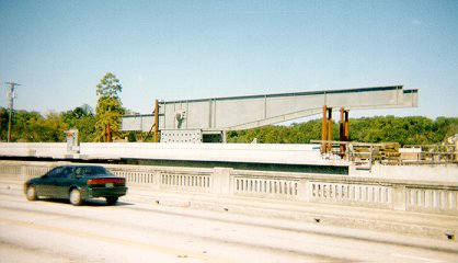
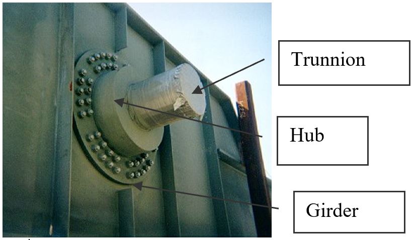
Figure 1 Trunnion-Hub-Girder (THG) assembly.
This is done by first immersing the trunnion in a cold medium such as dry-ice/alcohol mixture. After the trunnion reaches the steady-state temperature, that is, the temperature of the cold medium, the trunnion outer diameter contracts. The trunnion is taken out of the medium and slid through the hole of the hub (Figure 2).
Figure 2 Trunnion slid through the hub after contracting
When the trunnion heats up, it expands and creates an interference fit with the hub. In 1995, on one of the bridges in Florida, this assembly procedure did not work as designed. Before the trunnion could be inserted fully into the hub, the trunnion got stuck. Luckily the trunnion was taken out before it got stuck permanently. Otherwise, a new trunnion and hub would be needed to be ordered at a cost of $50,000. Coupled with construction delays, the total loss could have been more than a hundred thousand dollars.
Why did the trunnion get stuck? This was because the trunnion had not contracted enough to slide through the hole. Can you find out why?
A hollow trunnion of an outside diameter \(12.363^{\prime\prime}\) is to be fitted in a hub of an inner diameter \(12.358^{\prime\prime}\). The trunnion was put in dry-ice/alcohol mixture (temperature of the fluid - dry ice/alcohol mixture is \(- 108{^\circ}\text{F}\)) to contract the trunnion so that it can be slided through the hole of the hub. To slide the trunnion without sticking, a diametrical clearance of at least \(0.01^{\prime\prime}\) is required between the trunnion and the hub. Assuming the room temperature is \(80{^\circ}\text{F}\), is immersing it in dry-ice/alcohol mixture a correct decision?
Solution
To calculate the contraction in the diameter of the trunnion, the coefficient of linear thermal expansion at room temperature is used. In that case, the reduction, \({\Delta D}\) in the outer diameter of the trunnion is
\[\Delta D = D\alpha\Delta T\ \ \ (1)\]
where
\[D = \text{outer diameter of the trunnion,}\]
\[\alpha = \text{coefficient of linear thermal expansion at room temperature, and}\]
\[\Delta T = \text{change in temperature,}\]
Given
\[D = 12.363^{\prime\prime}\]
\[\alpha = 6.817 \times 10^{- 6}{in/in/}{^\circ}\text{F}\ \text{at}\ 80{^\circ}\text{F}\]
\[\begin{split} \Delta T&= T_{{fluid}} - T_{{room}}\\ &= - 108 - 80\\ &= - 188{^\circ}\text{F} \end{split}\] where
\[T_{{fluid}}= \text{temperature of dry-ice/alcohol mixture}\]
\[T_{{room}}= \text{room temperature}\]
the reduction in the trunnion outer diameter is given by
\[\begin{split} \Delta D &= (12.363)\left( 6.47 \times 10^{- 6} \right)\left( - 188 \right)\\ &=- 0.01504^{\prime\prime} \end{split}\]
So, the trunnion is predicted to reduce in diameter by \(0.01504^{\prime\prime}\). But is this enough reduction in diameter? As per specifications, he needs the trunnion to contract by
\[\begin{split} &= \text{trunnion outside diameter} - \text{hub inner diameter} + \text{diametral clearance} \\ &= 12.363^{\prime\prime} - 12.358^{\prime\prime} + 0.01^{\prime\prime}\\ &= 0.015^{\prime\prime} \end{split}\]
So, according to his calculations, immersing the steel trunnion in dry-ice/alcohol mixture gives the desired contraction of \(0.015^{\prime\prime}\) as we predict a contraction of \(0.01504^{\prime\prime}\).
But as shown in Figure 3, the coefficient of linear thermal expansion of steel decreases with temperature and is not constant over the range of temperature the trunnion goes through. Hence, Equation 1 would overestimate the thermal contraction.
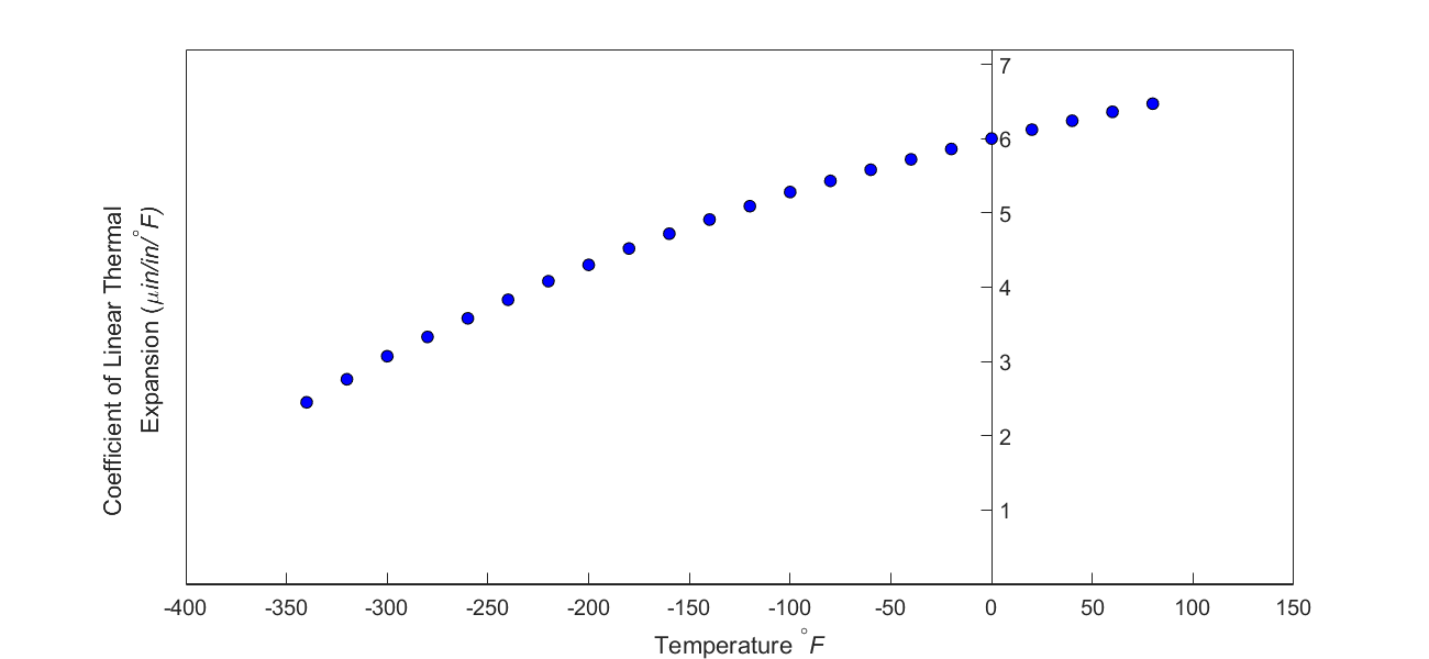
Figure 3 Varying coefficient of linear thermal expansion as a function of temperature for cast steel.
The contraction in the diameter for the trunnion for which the coefficient of linear thermal expansion varies as a function of temperature is given by
\[\Delta D = D\int_{T_{{room}}}^{T_{{fluid}}}{\alpha dT}\ \ \ (2)\]
So one needs to find the curve to find the coefficient of linear thermal expansion as a function of temperature. This curve is found by regression, where we best fit a polynomial through the data given in Table 1.
Table 1 Coefficient of linear thermal expansion as a function of temperature.
| Temperature | Coefficient of linear thermal expansion |
|---|---|
| \({^\circ}\text{F}\) | \({\mu }\text{in/in}/{^\circ}\text{F}\) |
| \(80\) | \(6.47\) |
| \(60\) | \(6.36\) |
| \(40\) | \(6.24\) |
| \(20\) | \(6.12\) |
| \(0\) | \(6.00\) |
| \(-20\) | \(5.86\) |
| \(-40\) | \(5.72\) |
| \(-60\) | \(5.58\) |
| \(-100\) | \(5.28\) |
| \(-120\) | \(5.09\) |
| \(-140\) | \(4.91\) |
| \(-160\) | \(4.72\) |
| \(-180\) | \(4.52\) |
| \(-200\) | \(4.30\) |
| \(-220\) | \(4.08\) |
| \(-240\) | \(3.83\) |
| \(-260\) | \(3.58\) |
| \(-280\) | \(3.33\) |
| \(-300\) | \(3.07\) |
| \(-320\) | \(2.76\) |
| \(-340\) | \(2.45\) |
Assuming that the coefficient of linear thermal expansion is related to temperature by a second-order polynomial,
\[\alpha = a_{0} + a_{1}T + a_{2}T^{2}\ \ \ (3)\]
Given the data points \(\left( \alpha_{1},T_{1} \right)\), \(\left( \alpha_{2},T_{2} \right)\), …..,\(\left( \alpha_{n},T_{n} \right)\) as in Figure 3 and Table 1, the sum of the square of the residuals (sum of the square of the differences between the observed and predicted values) is \[\begin{split} S_{r} &= \sum_{i = 1}^{n}\left( \alpha_{i} - \{ a_{0} + a_{1}T_{i} + a_{2}T_{i}^{2}\} \right)^{2}\\ &= \sum_{i = 1}^{n}\left( \alpha_{i} - a_{0} - a_{1}T_{i} - a_{2}T_{i}^{2} \right)^{2} \ \ \ (4) \end{split}\]
To minimize the value of the sum of the square of the residuals, we take the derivative with respect to each of the three unknown coefficients, \(a_0,\) \(a_1,\) and \(a_2\) to give
\[\begin{split} \frac{\partial S_{r}}{\partial a_{0}} &= \sum_{i = 1}^{n}{2\left( \alpha_{i} - a_{0} - a_{1}T_{i} - a_{2}T_{i}^{2} \right)}\left( - 1 \right)\\ &= 2\left\lbrack - \sum_{i = 1}^{n}\alpha_{i} + na_{0} + a_{1}\sum_{i = 1}^{n}T_{i} + a_{2}\sum_{i = 1}^{n}T_{i}^{2} \right\rbrack \end{split}\]
\[\begin{split} \frac{\partial S_{r}}{\partial a_{1}} &= \sum_{i = 1}^{n}{2\left( \alpha_{i} - a_{0} - a_{1}T_{i} - a_{2}T_{i}^{2} \right)}\left( - T_{i} \right)\\ &= 2\left\lbrack - \sum_{i = 1}^{n}{\alpha_{i}T_{i}} + a_{0}\sum_{i = 1}^{n}T_{i} + a_{1}\sum_{i = 1}^{n}{T_{i}}^{2} + a_{2}\sum_{i = 1}^{n}T_{i}^{3} \right\rbrack \end{split}\]
\[\begin{split} \frac{\partial S_{r}}{\partial a_{2}} &= \sum_{i = 1}^{n}{2\left( \alpha_{i} - a_{0} - a_{1}T_{i} - a_{2}T_{i}^{2} \right)}\left( - T_{i}^{2} \right)\\ &= 2\left\lbrack - \sum_{i = 1}^{n}{\alpha_{i}{T_{i}}^{2}} + a_{0}\sum_{i = 1}^{n}{T_{i}}^{2} + a_{1}\sum_{i = 1}^{n}T_{i}^{3} + a_{2}\sum_{i = 1}^{n}T_{i}^{4} \right\rbrack\ \ \ (5) \end{split}\]
Setting three partial derivatives in Equation (5) equal to zero gives,
\[na_{0} + a_{1}\sum_{i = 1}^{n}{T_{i} + a_{2}\sum_{i = 1}^{n}T_{i}^{2} = \sum_{i = 1}^{n}\alpha_{i}}\]
\[a_{0}\sum_{i = 1}^{n}T_{i} + a_{1}\sum_{i = 1}^{n}T_{i}^{2} + a_{2}\sum_{i = 1}^{n}T_{i}^{3} = \sum_{i = 1}^{n}{\alpha_{i}T_{i}}\]
\[a_{0}\sum_{i = 1}^{n}T_{i}^{2} + a_{1}\sum_{i = 1}^{n}T_{i}^{3} + a_{2}\sum_{i = 1}^{n}T_{i}^{4} = \sum_{i = 1}^{n}{\alpha_{i}T_{i}^{2}}\ \ \ (6)\]
The set of equations given by equations(6a), (6b), and (6c) are simultaneous linear equations. The number of data points in Figure (3) is \(24,\) as given in Table 1. Hence
\[n = 24\]
\[\sum_{i = 1}^{24}T_{i} = - 2860\]
\[\sum_{i = 1}^{24}T_{i}^{2} = 7.26 \times 10^{5}\]
\[\sum_{i = 1}^{24}T_{i}^{3} = - 1.86472 \times 10^{8}\]
\[\sum_{i = 1}^{24}T_{i}^{4} = 5.24357 \times 10^{10}\]
\[\sum_{i = 1}^{24}\alpha_{i} = 1.057 \times 10^{- 4}\]
\[\sum_{i = 1}^{24}\alpha_{i}T_{i} = - 1.04162 \times 10^{- 2}\]
\[\sum_{i = 1}^{24}\alpha_{i}T_{i}^{2} = 2.56799\]
\[\begin{split} &24a_{0} - 2860a_{1} + 7.26 \times 10^{5}a_{2} = 1.057 \times 10^{- 4}\\ &- 2860a_{0} + 7.26 \times 10^{5}a_{1} - 1.8647 \times 10^{8}a_{2} = - 1.04162 \times 10^{- 2}\\ &7.26 \times 10^{5}a_{0} - 1.86472 \times 10^{8}a_{1} + 5.24357 \times 10^{10}a_{2} = 2.56799 \end{split}\;\;\;\;\;\;\;\;\;\;\;\; (7)\]
In matrix form, the three simultaneous linear equations can be written as
\[\begin{bmatrix} 24 & - 2860 & 7.26 \times 10^{5} \\ - 2860 & 7.26 \times 10^{5} & - 1.86472 \times 10^{8} \\ 7.26 \times 10^{5} & - 1.86472 \times 10^{8} & 5.24357 \times 10^{10} \\ \end{bmatrix}\begin{bmatrix} a_{0} \\ a_{1} \\ a_{2} \\ \end{bmatrix} = \begin{bmatrix} 1.057 \times 10^{- 4} \\ - 1.04162 \times 10^{- 2} \\ 2.56799 \\ \end{bmatrix}\;\;\;\;\;\;\;\;\;\;\;\; (8)\]
Questions
(1) Can you now find the contraction in the trunnion outer diameter?
(2) Is the magnitude of contraction more than \(0.015^{\prime\prime}\) as required?
(3) If that is not the case, what if the trunnion were immersed in liquid nitrogen (boiling temperature=\(- 321{^\circ}\text{F}\))? Will that give enough contraction in the trunnion?
(4) Redo problem #1 using a third-order polynomial as the regression model. How much different is the estimate of contraction using the third-order polynomial?
(5) Find the optimum polynomial order to use for the regression model.
(6) Find the effect of the number of significant digits used in solving the set of the equations for problem #4 as you must have noticed that the order of the numbers in the coefficient matrix varies quite a bit.