Chapter 05.01: Prerequisites to Interpolation
Learning Objectives
After successful completion of this lesson, you should be able to:
1) define interpolation
2) interpolate using a straight line.
What is interpolation?
Many times, as given in Figure 1, data is given only at discrete points such as \(\left( x_{0},y_{0} \right),\) \(\left( x_{1},y_{1} \right)\), \(\displaystyle ......,\left( x_{n - 1},y_{n - 1} \right)\), \(\displaystyle \left( x_{n},y_{n} \right)\). So, how then does one find the value of \(y\) at any other value of \(x\)? Well, a continuous function \(f\left( x \right)\) may be used to represent the \(n + 1\) data values with \(f\left( x \right)\) passing through the \(n + 1\) points (Figure 1). Then one can find the value of \(y\) at any other value of \(x\). This curve fitting technique is called interpolation.
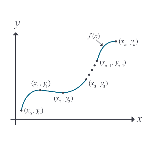
Figure 1. Interpolation of a function given at discrete points
The function \(f\left( x \right)\) chosen for interpolation is called the interpolant. The value of \(y\) at any other value of \(x\) that is not at the discrete data points is called the interpolated value. Of course, if \(x\) falls outside the domain of \(x\) for which the data is given, it is no longer interpolation and is called extrapolation.
So, what kind of function \(f\left( x \right)\) should one choose? A polynomial is a common choice for an interpolating function because polynomials are easy to
(A) evaluate,
(B) differentiate, and
(C) integrate
relative to other choices such as a trigonometric and exponential series. For example, given data points \((2,4), (3,10), (5,16)\), one may interpolate the data to
\[y\left( x \right) = a_{0} + a_{1}x + a_{2}x^{2},\ 2 \leq x \leq 5\]
Other examples of usable interpolants are
\[y\left( x \right) = a_{0} + a_{1}e^{x} + a_{2}e^{2x},\ 2 \leq x \leq 5\]
\[y\left( x \right) = a_{0} + a_{1}\sin x + a_{2}\sin2x,\ 2 \leq x \leq 5\]
The problem hence reduces to finding the unknown coefficients, \(a_{0},\ \ a_{1},\) and \({a}_{2}\). Once these are found, one can estimate the value of the dependent variable value \(y\) at any value of \(x\) within the bounds of the \(x\) values.
Learning Objectives
After successful completion of this lesson, you should be able to:
1) derive why a polynomial of degree n or less that passes through n + 1 data points is unique.
Proof for a unique polynomial of degree \(n\) or less passes through \(n+1\) data points.
Let us use proof by contradiction. If the polynomial is not unique, then at least two polynomials of order \(n\) or less pass through the \(n + 1\) data points.
Assume two polynomials \(P_{n}\left( x \right)\) and \(Q_{n}\left( x \right)\) go through \(n + 1\) data points,
\[\left( x_{0},y_{0} \right),\left( x_{1},y_{1} \right),\ldots,\left( x_{n},y_{n} \right)\]
Then
\[R_{n}\left( x \right) = P_{n}\left( x \right) - Q_{n}\left( x \right)\;\;\;\;\;\;\;\;\;\;\;\; (1)\]
Since \(P_{n}\left( x \right)\)and \(Q_{n}\left( x \right)\) pass through all the \(n + 1\) data points,
\[P_{n}\left( x_{i} \right) = Q_{n}\left( x_{i} \right), i = 0,\ldots,n\;\;\;\;\;\;\;\;\;\;\;\; (2)\]
Hence
\[R_{n}\left( x_{i} \right) = P_{n}(x_{i}) - Q_{n}\left( x_{i} \right) = 0, i = 0,\ldots,n\;\;\;\;\;\;\;\;\;\;\;\; (3)\]
The \(n^{{th}}\) order polynomial \(R_{n}\left( x \right)\) has \(n + 1\) zeros. A polynomial of order n can have \(n + 1\) zeros only if it is identical to a zero polynomial, that is,
\[R_{n}\left( x \right) \equiv 0\;\;\;\;\;\;\;\;\;\;\;\; (4)\]
Hence from Equation (1)
\[P_{n}\left( x \right) \equiv Q_{n}\left( x \right)\]
Example
Show that a unique polynomial of degree \(2\) or less passes through \(3\) data points
Solution
Let us use proof by contradiction. If the polynomial is not unique, then at least two polynomials of order \(3\) or less pass through the \(3\) data points.
Assume two polynomials \(P_{2}\left( x \right)\) and \(Q_{2}\left( x \right)\) go through \(3\) data points (Figure 1),
\[\left( x_{0},y_{0} \right),\left( x_{1},y_{1} \right),\left( x_{2},y_{2} \right)\]
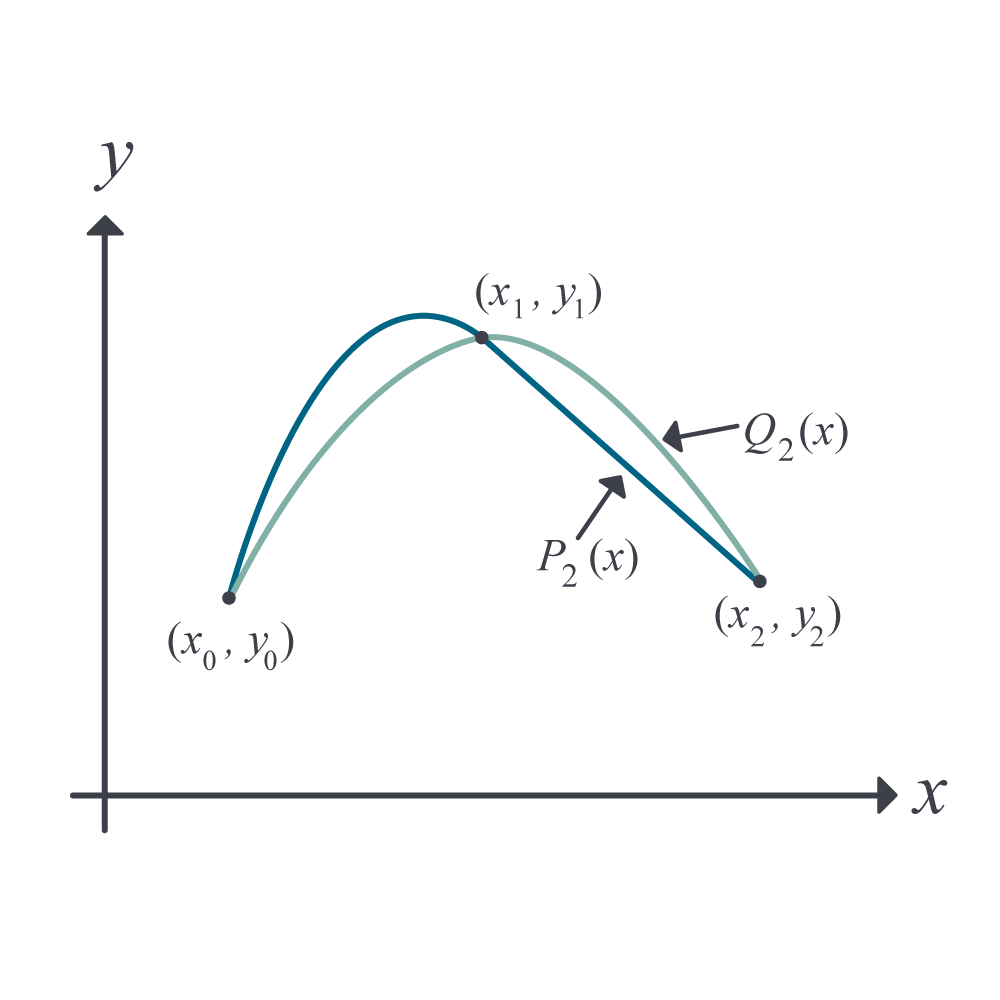
Figure 1. Interpolating polynomials through three points.
Then
\[R_{2}\left( x \right) = P_{2}\left( x \right) - Q_{2}\left( x \right)\;\;\;\;\;\;\;\;\;\;\;\; (E1.1)\]
Since \(P_{2}\left( x \right)\)and \(Q_{2}\left( x \right)\) pass through all the \(3\) data points,
\[P_{2}\left( x_{i} \right) = Q_{2}\left( x_{i} \right), i = 0,\ 1,\ 2\;\;\;\;\;\;\;\;\;\;\;\; (E1.2)\]
Hence
\[R_{2}\left( x_{i} \right) = P_{2}(x_{i}) - Q_{2}\left( x_{i} \right) = 0, i = 0,\ 1,\ 2\;\;\;\;\;\;\;\;\;\;\;\; (E1.3)\]
Let \(R_{2}\left( x \right)\) be written as
\[R_{2}\left( x \right) = a_{0} + a_{1}x + a_{2}x^{2}.\;\;\;\;\;\;\;\;\;\;\;\; (E1.4)\]
The \(2^{{nd}}\) order polynomial \(R_{2}\left( x \right)\) has \(3\) zeros and these zeros are at \(x_1\), \(x_2\), and \(x_3\). Then from Equation (E1.4)
\[\begin{split} R_{2}\left( x_{1} \right) = a_{0} + a_{1}x_{1} + a_{2}x_{1}^{2} &= 0\\ R_{2}\left( x_{2} \right) = a_{0} + a_{1}x_{2} + a_{2}x_{2}^{2} &= 0\\ R_{2}\left( x_{3} \right) = a_{0} + a_{1}x_{3} + a_{2}x_{3}^{2} &= 0\end{split}\;\;\;\;\;\;\;\;\;\;\;\; (E1.5)\]
which in the matrix form gives
\[\begin{bmatrix} 1 & x_{1} & x_{1}^{2} \\ 1 & x_{2} & x_{2}^{2} \\ 1 & x_{3} & x_{3}^{2} \end{bmatrix}\begin{bmatrix} a_{0} \\ a_{1} \\ a_{2} \\ \end{bmatrix} = \begin{bmatrix} 0 \\ 0 \\ 0 \\ \end{bmatrix}\;\;\;\;\;\;\;\;\;\;\;\; (E1.6)\]
The above set of equations has a trivial solution, that is, \(a_{1} = a_{2} = a_{3} = 0\). But is this the only solution? That is true if the coefficient matrix is invertible.
The determinant of the coefficient matrix can be found symbolically with the forward elimination steps of Naïve Gauss elimination to give
\[\begin{split} \det\begin{bmatrix} 1 & x_{1} & x_{1}^{2} \\ 1 & x_{2} & x_{2}^{2} \\ 1 & x_{3} & x_{3}^{2} \\ \end{bmatrix} &= x_{2}x_{3}^{2} - x_{2}^{2}x_{3} - x_{1}x_{3}^{2} + x_{1}^{2}x_{3} + x_{1}x_{2}^{2} - x_{1}^{2}x_{2}\\ &= (x_{1} - x_{2})(x_{2} - x_{3})(x_{3} - x_{1})\end{split}\;\;\;\;\;\;\;\;\;\;\;\; (E1.7)\]
Since
\[x_{1} \neq x_{2} \neq x_{3}\]
the determinant is non-zero. Hence the coefficient matrix is invertible. \(a_{1} = a_{2} = a_{3} = 0\) is the only solution, that is, \(R_{2}\left( x \right) \equiv 0\) giving \(P_{2}\left( x \right) \equiv Q_{2}\left( x \right)\) showing that the polynomial has to be unique.
Multiple Choice Test
(1). The number of different polynomials that can go through two fixed data points \(\left( x_{1},y_{1} \right)\) and \(\left( x_{2},y_{2} \right)\) is
(A) \(0\)
(B) \(1\)
(C) \(2\)
(D) infinite
(2). Given \(n+1\) data pairs, a unique polynomial of degree __________________ passes through \(n + 1\) data points.
(A) \(n + 1\)
(B) \(n + 1\) or less
(C) \(n\)
(D) \(n\) or less
(3). The following function(s) can be used for interpolation:
(A) polynomial
(B) exponential
(C) trigonometric
(D) all of the above
(4). Polynomials are the most commonly used functions for interpolation because they are easy to
(A) evaluate
(B) differentiate
(C) integrate
(D) evaluate, differentiate and integrate
(5). Given \(n + 1\) data points \(\left( x_{0},y_{0} \right),\left( x_{1},y_{1} \right),......,\left( x_{n - 1},y_{n - 1} \right),\left( x_{n},y_{n} \right)\), assume you pass a function \(f(x)\) through all the data points. If now the value of the function \(f(x)\) is required to be found outside the range of the given \(x\)-data, the procedure is called
(A) extrapolation
(B) interpolation
(C) guessing
(D) regression
(6). Given three data points \((1,6)\), \((3,28)\), and \((10, 231)\), it is found that the function \(y = 2x^{2} + 3x + 1\) passes through the three data points. Your estimate of \(y\) at \(x = 2\) is most nearly
(A) \(6\)
(B) \(15\)
(C) \(17\)
(D) \(28\)
For complete solution, go to
http://nm.mathforcollege.com/mcquizzes/05inp/quiz_05inp_background_solution.pdf