Chapter 07.00: Physical Problem for Integration
Summary
The upward velocity of a rocket is given. To find the distance covered by the rocket requires integration.
Modeling
A rocket is going vertically up and expels fuel at a velocity \(2000\ \text{m/s}\) at a consumption rate of \(2100\ \text{kg/s}\). The initial mass of the rocket is \(140,000\ \text{kg}\). If the rocket starts from rest at \(t = 0\) seconds, how can I calculate the vertical distance covered by the rocket from \(t = 8\) to \(t = 30\) seconds?
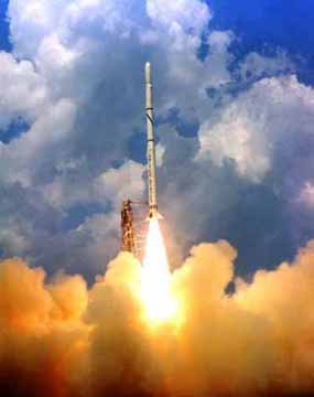
Figure 1 A rocket launched into space
If
\[m_{0} = \text{initial mass of rocket at}\ t = 0\ \text{(kg)}\]
\[q = \text{rate at which fuel is expelled (kg/sec)}\]
\[u = \text{velocity at which the fuel is being expelled (m/s)}\]
Then since fuel is expelled from the rocket, the mass of the rocket keeps decreasing with time. The mass of the rocket, \(m\) at any time \(t\)
\[m = m_{0} - {qt}\;\;\;\;\;\;\;\;\;\;\;\; (1)\]
The forces on the rocket at any time are found by applying Newton’s second law of motion. Then
\[\sum_{}^{}{F = ma}\;\;\;\;\;\;\;\;\;\;\;\; (2)\]
gives
\[{uq} - mg = ma\;\;\;\;\;\;\;\;\;\;\;\; (3)\]
Substituting Equation (1) in Equation (3) gives
\[{uq} - (m_{0} - qt)g = (m_{0} - qt)a\;\;\;\;\;\;\;\;\;\;\;\; (4)\]
where
\[g = \text{acceleration due to gravity (m/s}^{2})\]
Equation (4) is simplified to
\[a = \frac{{uq}}{m_{0} - {qt}} - g\;\;\;\;\;\;\;\;\;\;\;\; (5)\]
\[\frac{d^{2}x}{dt^{2}} = \frac{{uq}}{m_{0} - {qt}} - g\;\;\;\;\;\;\;\;\;\;\;\; (6)\]
\[\frac{{dx}}{{dt}} = - u\ln(m_{0} - qt) - gt + C\;\;\;\;\;\;\;\;\;\;\;\; (7)\]
Since the rocket starts from rest
\[\frac{{dx}}{{dt}} = 0\ \text{at}\ t = 0\]
\[0 = u\ln(m_{0}) + C\]
\[C = u\ln(m_{0})\]
Hence
\[\begin{split} \frac{{dx}}{{dt}} &= - u\ln(m_{0} - qt) - gt + u\ln(m_{0})\\ &= u\ln\left( \frac{m_{0}}{m_{0} - {qt}} \right) - {gt}\;\;\;\;\;\;\;\;\;\;\;\; (8) \end{split}\]
Then the distance covered by the rocket from \(t = t_{0}\) to \(t = t_{1}\) is,
\[x = \int_{t_{0}}^{t_{1}}{\left\lbrack u\ln\left( \frac{m_{0}}{m_{0} - {qt}} \right) - {gt} \right\rbrack{dt}}\;\;\;\;\;\;\;\;\;\;\;\; (9)\]
Let us substitute the values into the above equation. A rocket is going vertically up and expels fuel at a velocity \(2000\ \text{m/s}\) at a consumption rate of \(2100\ \text{kg/s}\). The initial mass of the rocket is \(140,000\ \text{kg}\). If the rocket starts from rest at \(t = 0\) seconds, how can I calculate the vertical distance covered by the rocket from \(t = 8\) to \(t = 30\) seconds?
Substituting
\[u = 2000\ \text{m/s}\]
\[m_{0} = 140000\ \text{kg}\]
\[q = 2100\ \text{kg/s}\]
\[g = 9.8\ \text{m/s}^2\]
\[t_{0} = 8\ \text{s}\]
\[t_{1} = 30\ \text{s}\]
\[x = \int_{8}^{30}{\left( 2000\ln\left\lbrack \frac{140000}{140000 - 2100t} \right\rbrack - 9.8t \right){dt}}\]
Summary
The number of sheets in a roll of toilet paper are sampled at a factory. Even if the number of the sheets in every chosen sample turns out to be what is advertised or more, the probability of every roll having the advertised number or more sheets is not \(100\%\). To find out this probability requires numerical integration.
Modeling
An industrial engineer works as a quality control engineer for a company making toilet paper. The company advertises that every roll of toilet paper has at least \(250\) sheets. It is the industrial (quality) engineer’s responsibility to validate this claim by sampling rolls off of the assembly line and determining the probability (that is, confidence) that the company can make a claim. Note that validating the claim is important to avoid frivolous lawsuits associated with false advertising.
Let us assume that the number of sheets in a roll of toilet paper, \(y\), is governed by the normal probability distribution (see figure on next page), that is,
\[y \sim N(\mu,\sigma^{2})\;\;\;\;\;\;\;\;\;\;\;\; (1)\]
where N is a normal random variable described by its mean, \(\mu\) , and standard deviation, \(\sigma\). The probability distribution function of the normal random variable \(y\) is
\[f(y) = \frac{1}{\sigma\sqrt{2\pi}}e^{-(1/2)\left\lbrack y - \mu)/\sigma \right\rbrack^{2}}\;\;\;\;\;\;\;\;\;\;\;\; (2)\]
and is shown in Figure 1.
Note that the previously described normal probability density function was first derived by Abraham de Moivre in 1733 in his book called The Doctrine of Chance. Initially, the discovery went unnoticed until it was re-derived by Laplace and Gauss about 50 years later. Hence, it is often called the Gaussian distribution. The normal probability distribution, which is a continuous distribution, is derived from the binomial probability distribution, which is a discrete distribution. The discrete binomial distribution is given below
\[f(y) =\frac{n!}{k!\left( n - k \right)!}p^{k}\left( 1 - p \right)^{n - k}\;\;\;\;\;\;\;\;\;\;\;\; (3)\]
where \(n\) is the number of samples and \(k\) is the number of successes with a probability of \(p\). When \(n\) is large, the binomial distribution approaches the normal distribution. In fact, when \(n\) is greater than or equal to \(6\), the normal distribution is an excellent approximation to the binomial distribution (Figure 2).
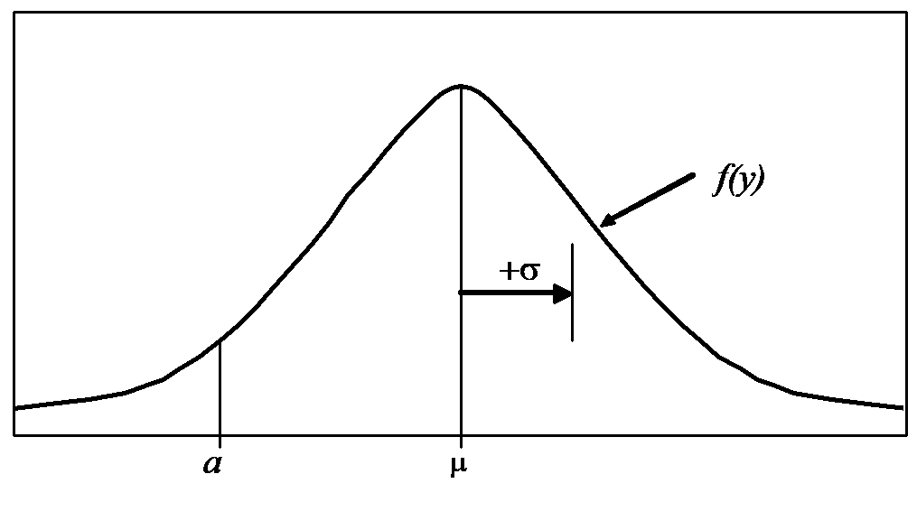
Figure 1 Probability distribution function,
\(\displaystyle f(y) = \frac{1}{\sigma\sqrt{2\pi}}e^{- (1/2)\left\lbrack y - \mu)/\sigma \right\rbrack^{2}}\)
The actual proof that the binomial distribution approaches the normal distribution involves a special case of the central limit theorem and is beyond the scope of this problem. Furthermore, the derivation also involves the inclusion of a continuity correction factor.
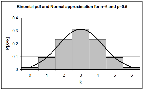
Figure 2 Binomial pdf and normal approximation for \(n = 6\) and \(p = 0.5\)
Since the quality engineer cannot sample every roll of toilet paper and count the number of sheets, the mean and standard deviation are estimated based on a sample size of \(n\) rolls of toilet paper. The mean, \(\bar{y}\), and standard deviation, \(s\), of the sample (that is, the sample mean and sample standard deviation) are estimates of the actual mean, \(\mu\), and standard deviation, \(\sigma\), and are given by
\[\bar{y} = \frac{\displaystyle \sum_{i = 1}^{n}y_{i}}{n} \approx \mu\;\;\;\;\;\;\;\;\;\;\;\; (4)\]
\[s = \sqrt{\frac{\displaystyle \sum_{i = 1}^{n}\left( y_{i} - \bar{y} \right)^{2}}{n - 1}} \approx \sigma\;\;\;\;\;\;\;\;\;\;\;\; (5)\]
where \(n\) is the number of samples (that is, rolls of toilet paper). The probability that the number of sheets in a roll is greater than or equal to some specified number, \(a\), is the area under the probability density function (that is, integral) from \(a\) to \(\infty\), and is given by
\[\begin{split} P(y \geq a) &= \int_{a}^{\infty}{f(y)dy}\\ &= \int_{a}^{\infty}{\frac{1}{\sigma\sqrt{2\pi}}e^{- (1/2)\left\lbrack (y - \mu)/\sigma \right\rbrack^{2}}{dy}}\;\;\;\;\;\;\;\;\;\;\;\; (6) \end{split}\]
Note that the result of Equation (6) is a number from \(0\) to \(1\) that correlates to a \(0\%\) to \(100\%\) probability, respectively.
A co-operative education student working for an industrial (quality) engineer samples \(10\) rolls of toilet paper every week and determines that the number of sheets in each roll is
| Roll | Number of sheets |
|---|---|
| \(1\) | \(253\) |
| \(2\) | \(250\) |
| \(3\) | \(251\) |
| \(4\) | \(252\) |
| \(5\) | \(253\) |
| \(6\) | \(253\) |
| \(7\) | \(252\) |
| \(8\) | \(254\) |
| \(9\) | \(252\) |
| \(10\) | \(252\) |
The industrial (quality) engineer calculates the following mean and standard deviation of the sample of 10 rolls of toilet paper.
\[\bar{y} = \frac{253 + 250 + 251 + 252 + 253 + 253 + 252 + 254 + 252 + 252}{10} = 252.2 \approx \mu\]
\[s = \sqrt{\frac{\begin{matrix} \ &\left( 253 - 252.2 \right)^{2} + \left( 250 - 252.2 \right)^{2} + \left( 251 - 252.2 \right)^{2} + \\ \ &\left( 252 - 252.2 \right)^{2} + \left( 253 - 252.2 \right)^{2} + \left( 253 - 252.2 \right)^{2} + \\ \ &\left( 252 - 252.2 \right)^{2} + \left( 254 - 252.2 \right)^{2} + \left( 252 - 252.2 \right)^{2} + \left( 252 - 252.2 \right)^{2} \\ \end{matrix}}{10 - 1}} = 1.135 \approx \sigma\]
Using Equation (6), the probability that the number of sheets in a roll is greater than or equal to \(250\) sheets is
\[P(y \geq 250) = \int_{250}^{\infty}{\frac{1}{1.135\sqrt{2\pi}}e^{- (1/2)\left\lbrack (y - 252.2)/1.135 \right\rbrack^{2}}{dy}}\]
\[P(y \geq 250) = \int_{250}^{\infty}{0.3515e^{- 0.3881(y - 252.2)^{2}}{dy}}\]
\[P(y \geq 250) = ??\]
Questions
(1) Although all the rolls have more than \(250\) sheets, why do we not get a \(100\%\) probability that all the rolls have \(250\) sheets or more?
(2) Change one of the data points to \(248\) sheets and rework the problem.
(3) To find the integral numerically in Equation (6), one may substitute infinity by \(5\). How will you justify this substitution quantitatively?
Summary
To find the diametrical contraction during shrink-fitting in a trunnion requires one to first find how the coefficient of linear thermal expansion of steel is related to temperature. The relation may be given through a second-order polynomial. This model is then used in integration to find the diametrical contraction.
Modeling
To make the fulcrum (Figure 1) of a bascule bridge, a long hollow steel shaft called the trunnion is shrink fit into a steel hub. The resulting steel trunnion-hub assembly is then shrink fit into the girder of the bridge.
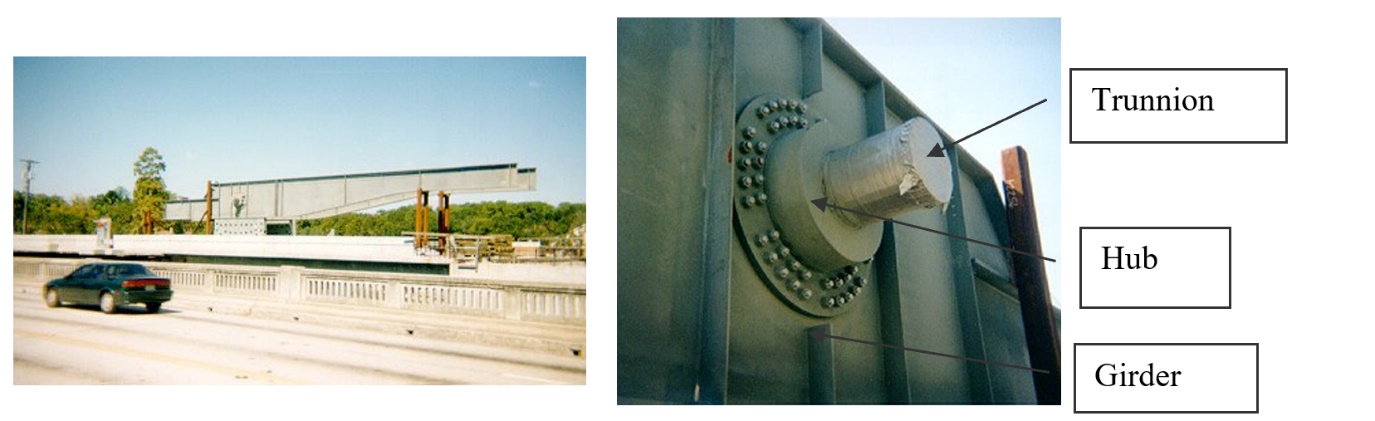
Figure 1 Trunnion-Hub-Girder (THG) assembly.
This is done by first immersing the trunnion in a cold medium such as a dry-ice/alcohol mixture. After the trunnion reaches the steady-state temperature, that is, the temperature of the cold medium, the trunnion outer diameter contracts. The trunnion is taken out of the medium and slid though the hole of the hub (Figure 2).
When the trunnion heats up, it expands and creates an interference fit with the hub. In 1995, on one of the bridges in Florida, this assembly procedure did not work as designed. Before the trunnion could be inserted fully into the hub, the trunnion got stuck. Luckily the trunnion was taken out before it got stuck permanently. Otherwise, a new trunnion and hub would be needed to be ordered at a cost of $50,000. Coupled with construction delays, the total loss could have been more than a hundred thousand dollars.
Why did the trunnion get stuck? This failure took place because the trunnion had not contracted enough to slide through the hole. Can you find out why?
A hollow trunnion of outside diameter \({12.36}{3}^{\prime\prime}\) is to be fitted in a hub of inner diameter \(12.358^{\prime\prime}\). The trunnion was put in a dry ice/alcohol mixture (temperature of the fluid - dry ice/alcohol mixture is \(- 108{^\circ}\text{F}\)) to contract the trunnion so that it can be slid through the hole of the hub. To slide the trunnion without sticking, a diametrical clearance of at least \(0.01^{\prime\prime}\) is required between the trunnion and the hub. Assuming the room temperature is \(80{^\circ}\text{F}\), is immersing it in a dry-ice/alcohol mixture a correct decision?
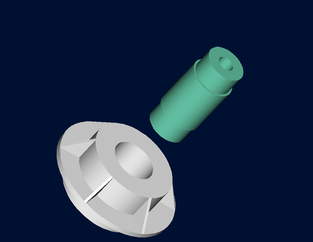
Figure 2 Trunnion slided through the hub after contracting
To calculate the contraction in the diameter of the trunnion, the coefficient of linear thermal expansion at room temperature is used. In that case, the reduction, \({\Delta D}\) in the outer diameter of the trunnion is
\[\Delta D = D\alpha\Delta T\;\;\;\;\;\;\;\;\;\;\;\; (1)\]
where
\[D = \text{outer diameter of the trunnion,}\]
\[\alpha =\text{coefficient of linear thermal expansion at room temperature, and}\]
\[\Delta T =\text{change in temperature,}\]
Given
\[D = 12.363^{\prime\prime}\]
\[\alpha = 6.817 \times 10^{- 6}\ \text{in/in/}{^\circ}\text{F}\ \text{at}\ 80{^\circ}\text{F}\]
\[\begin{split} \Delta T &=T_{{fluid}} - T_{{room}}\\ &= - 188{^\circ}\text{F} \end{split}\]
where
\[T_{{fluid}} = \text{temperature of dry-ice/alcohol mixture,}\]
\[T_{{room}}= \text{room temperature,}\]
the reduction in the trunnion outer diameter is given by
\[\begin{split} \Delta D &= (12.363)\left( 6.47 \times 10^{- 6} \right)\left( - 188 \right)\\ &= - 0.01504^{\prime\prime} \end{split}\]
So the trunnion is predicted to reduce in diameter by \(0.01504^{\prime\prime}\). But is this enough reduction in diameter? As per specifications, he needs the trunnion to contract by
\[\begin{split} &= \text{trunnion outside diameter} - \text{hub inner diameter} + \text{diametral clearance}\\ &= 12.363^{\prime\prime} - 12.358^{\prime\prime} + 0.01^{\prime\prime}\\ &= 0.015^{\prime\prime} \end{split}\]
So, according to his calculations, immersing the steel trunnion in a dry-ice/alcohol mixture gives the desired contraction of \(0.015^{\prime\prime}\) as we predict a contraction of \(0.01504^{\prime\prime}\).
But as shown in Figure 3, the coefficient of linear thermal expansion of steel decreases with temperature and is not constant over the range of temperature the trunnion goes through. Hence the above formula (Equation (1)) would overestimate the thermal contraction.
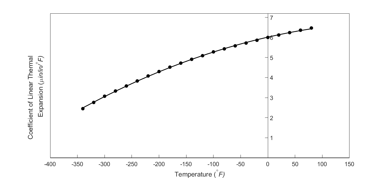 Figure 3 Varying coefficient of linear thermal expansion as a
function of temperature for cast steel.
Figure 3 Varying coefficient of linear thermal expansion as a
function of temperature for cast steel.
The contraction in the diameter for the trunnion for which the thermal expansion coefficient varies as a function of temperature is given by
\[\Delta D = D\int_{T_{{room}}}^{T_{{fluid}}}{\alpha dT}\;\;\;\;\;\;\;\;\;\;\;\; (2)\]
Note that Equation (2) reduces to Equation (1) if the coefficient of thermal expansion is assumed to be constant. In Figure 3, the coefficient of linear thermal expansion of typical cast steel is approximated by a second-order polynomial as
\[\alpha = - 1.2278 \times 10^{- 11}T^{2} + 6.1946 \times 10^{- 9}T + 6.0150 \times 10^{- 6}\;\;\;\;\;\;\;\;\;\;\;\; (3)\]
From Equations (2) and (3)
\[\Delta D = 12.363\int_{80}^{- 108}{\left( - 1.2278 \times 10^{- 11}T^{2} + 6.1946 \times 10^{- 9}T + 6.015 \times 10^{- 6} \right){dT}}\;\;\;\;\;\;\;\;\;\;\;\; (4)\]
Questions
(1) Can you now find the contraction of the trunnion outer diameter?
(2) Is the magnitude of contraction more than \(0.015^{\prime\prime}\) as required?
(3) If that is not the case, what if the trunnion were immersed in liquid nitrogen (boiling temperature=\(- 321{^\circ}\text{F}\))? Will that give enough contraction in the trunnion?
(4) Rather than regressing the data to a second-order polynomial so that one can find the contraction in the trunnion outer diameter, how would you use the trapezoidal rule of integration for unequal segments? What is the relative difference between the two results? The data for the coefficient of linear thermal expansion as a function of temperature is given below.
Table 1 coefficient of linear thermal expansion as a function of temperature.
| Temperature | Coefficient of Thermal Expansion |
|---|---|
| \({^\circ}\text{F}\) | \(\mu\text{in/in/}{^\circ}\text{F}\) |
| \(80\) | \(6.47\) |
| \(60\) | \(6.36\) |
| \(40\) | \(6.24\) |
| \(20\) | \(6.12\) |
| \(0\) | \(6.00\) |
| \(-20\) | \(5.86\) |
| \(-40\) | \(5.72\) |
| \(-60\) | \(5.58\) |
| \(-80\) | \(5.43\) |
| \(-100\) | \(5.28\) |
| \(-120\) | \(5.09\) |
| \(-140\) | \(4.91\) |
| \(-160\) | \(4.72\) |
| \(-180\) | \(4.52\) |
| \(-200\) | \(4.30\) |
| \(-220\) | \(4.08\) |
| \(-240\) | \(3.83\) |
| \(-260\) | \(3.58\) |
| \(-280\) | \(3.33\) |
| \(-300\) | \(3.07\) |
| \(-320\) | \(2.76\) |
| \(-340\) | \(2.45\) |
The second-order polynomial is derived using regression analysis which is another mathematical process where numerical methods are employed. Regression analysis approximates discrete data such as the coefficient of linear thermal expansion vs. temperature data as a continuous function. This is an excellent example of where one has to use numerical methods for more than one process to solve a real-life problem.