Chapter 04.00: Physical Problem for Simultaneous Linear Equations
Summary
To find the velocity profile of a rocket requires a solution of simultaneous linear equations.
Modeling
The upward velocity of a rocket is given at three different times in the following table
| Time, t | Velocity, v |
|---|---|
| \(\text{s}\) | \(\text{m/s}\) |
| \(5\) | \(106.8\) |
| \(8\) | \(177.2\) |
| \(12\) | \(279.2\) |
The velocity data is approximated by a polynomial as
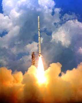
Figure 1 A rocket launched into space
\[v\left( t \right) = at^{2} + bt + c, \ 5 \leq t \leq 12.\;\;\;\;\;\;\;\;\;\;\;\; (1)\]
Set up the equations in matrix form to find the coefficients \(a,\ b,\ c\) of the velocity profile.
The polynomial is going through three data points \(\left( t_{1},v_{1} \right),\left( t_{2},v_{2} \right)\text{, and }\left( t_{3},v_{3} \right)\) where from the above table
\[t_{1} = 5,v_{1} = 106.8\]
\[t_{2} = 8,v_{2} = 177.2\]
\[t_{3} = 12,v_{3} = 279.2\]
Requiring that \(v\left( t \right) = at^{2} + bt + c\) passes through the three data points gives
\[\begin{split} v\left( t_{1} \right) &= v_{1} = at_{1}^{2} + bt_{1} + c\\ v\left( t_{2} \right) &= v_{2} = at_{2}^{2} + bt_{2} + c\\ v\left( t_{3} \right) &= v_{3} = at_{3}^{2} + bt_{3} + c \end{split}\]
Substituting the data \(\left( t_{1},\ v_{1} \right),\ \left( t_{2},\ v_{2} \right),\ \left( t_{3},\ v_{3} \right)\) gives
\[\begin{split} a\left( 5^{2} \right) + b\left( 5 \right) + c &= 106.8\\ a\left( 8^{2} \right) + b\left( 8 \right) + c &= 177.2\\ a\left( 12^{2} \right) + b\left( 12 \right) + c &= 279.2 \end{split}\]
or
\[\begin{split} 25a + 5b + c &= 106.8\\ 64a + 8b + c &= 177.2\\ 144a + 12b + c &= 279.2 \end{split}\]
This set of equations can be rewritten in the matrix form as
\[\begin{bmatrix} 25a + & 5b + & c \\ 64a + & 8b + & c \\ 144a + & 12b + & c \\ \end{bmatrix} = \begin{bmatrix} 106.8 \\ 177.2 \\ 279.2 \\ \end{bmatrix}\]
The above equation can be written as a linear combination as follows
\[a\begin{bmatrix} 25 \\ 64 \\ 144 \\ \end{bmatrix} + b\begin{bmatrix} 5 \\ 8 \\ 12 \\ \end{bmatrix} + c\begin{bmatrix} 1 \\ 1 \\ 1 \\ \end{bmatrix} = \begin{bmatrix} 106.8 \\ 177.2 \\ 279.2 \\ \end{bmatrix}\]
and further using matrix multiplications gives
\[\begin{bmatrix} 25 & 5 & 1 \\ 64 & 8 & 1 \\ 144 & 12 & 1 \\ \end{bmatrix}\ \begin{bmatrix} a \\ b \\ c \\ \end{bmatrix} = \begin{bmatrix} 106.8 \\ 177.2 \\ 279.2 \\ \end{bmatrix}\]
The solution of the above three simultaneous linear equations will give the value of \(a,b,c\).
Questions
(1) Solve for the values of \(a,b,c\).
(2) Verify if you get back the value of the velocity data at \(t=5\ \text{s}\).
(3) Estimate the velocity of the rocket at \(t=7.5\ \text{s}\)?
(4) Estimate the acceleration of the rocket at \(t=7.5\ \text{s}\)?
(5) Estimate the distance covered by the rocket between \(t=5.5\ \text{s}\) and \(8.9\ \text{s}\).
(6) If the following data is given for the velocity of the rocket as a function of time, and you are asked to use a quadratic polynomial to approximate the velocity profile to find the velocity at \(t=16\ \text{s}\), what data points would you choose and why?
| t | v(t) |
|---|---|
| \(\text{s}\) | \(\text{m/s}\) |
| \(0\) | \(0\) |
| \(10\) | \(227.04\) |
| \(15\) | \(362.78\) |
| \(20\) | \(517.35\) |
| \(22.5\) | \(602.97\) |
| \(30\) | \(901.67\) |
Summary
A pressure vessel made of a compounded cylinder has a higher capability to handle internal pressure over a single cylinder. To find this capability, one has to solve a set of simultaneous linear equations.
Modeling
A pressure vessel can only be subjected to an amount of internal pressure that is limited by the strength of the material used. For example, take a pressure vessel of an internal radius of \(a = 5^{\prime\prime}\) and outer radius, \(b = 8^{\prime\prime}\), made of ASTM 36 steel (yield strength of ASTM 36 steel is 36 ksi). How much internal pressure can this pressure vessel take before it is considered to have failed?
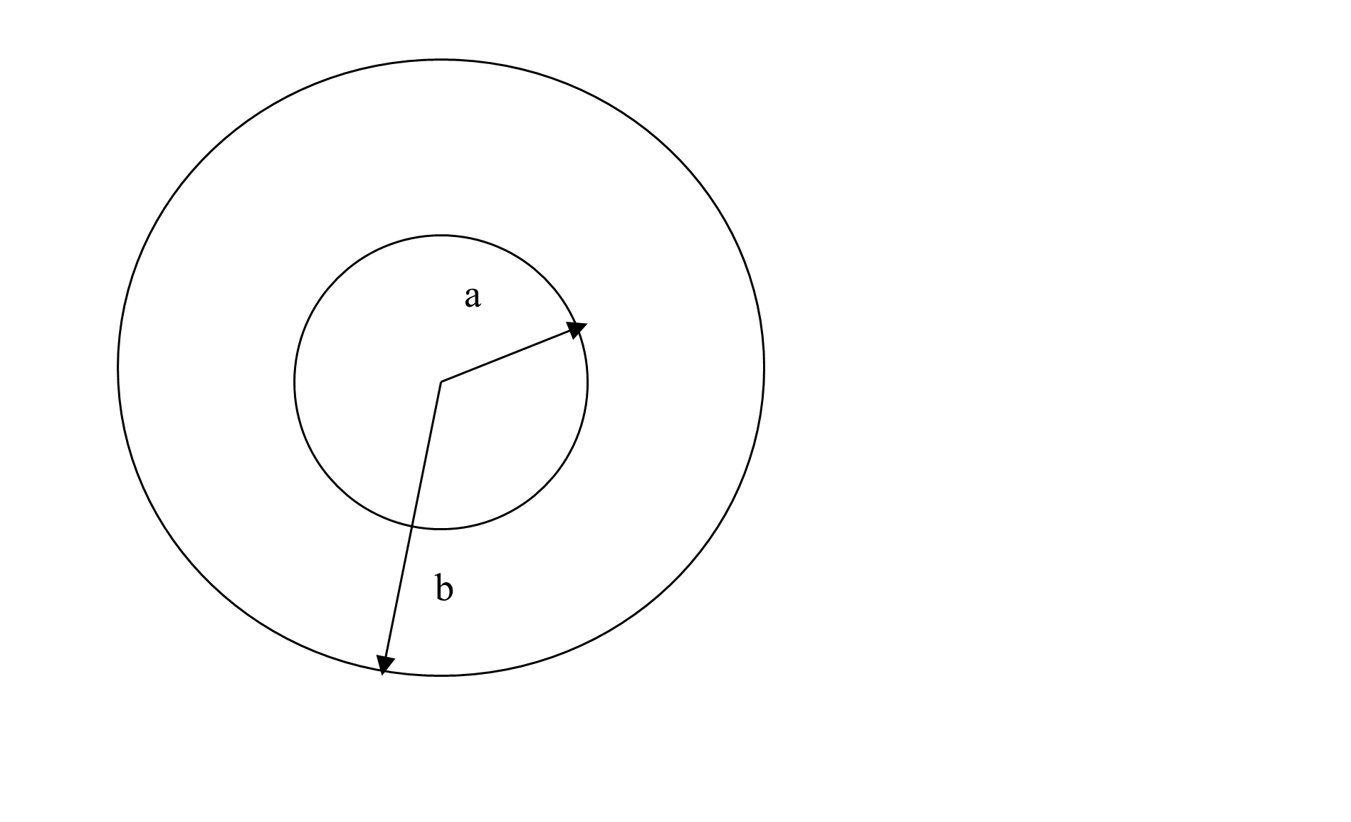
Figure 1 A single-cylinder pressure vessel with internal radius, \(a\) and outer radius, \(b\).
The hoop and radial stress in a cylindrical pressure vessel is given by [1]
\[\sigma_{r} = \frac{a^{2}p_{i}}{b^{2} - a^{2}}\left( 1 - \frac{b^{2}}{r^{2}} \right)\;\;\;\;\;\;\;\;\;\;\;\; (1)\]
\[\sigma_{\theta} = \frac{a^{2}p_{i}}{b^{2} - a^{2}}\left( 1 + \frac{b^{2}}{r^{2}} \right)\;\;\;\;\;\;\;\;\;\;\;\; (2)\]
The maximum normal stress anywhere in the cylinder is the hoop stress at the inner radius, \(a\)
\[{\left. \ \sigma_{\theta} \right|i\left( \frac{b^{2} + a^{2}}{b^{2} - a^{2}} \right)}_{\max}\;\;\;\;\;\;\;\;\;\;\;\; (3)\]
Assuming a factor of safety of 2, while the yield strength is given as 36 ksi,
\[\frac{36 \times 10^{3}}{2} = p_{i}\left( \frac{8^{2} + 5^{2}}{8^{2} - 5^{2}} \right)\]
\[p_{i} = 7.887{ksi}\]
You can see from Equation (3) that even for \(b > > a\), the maximum internal pressure one can apply is only \(p_{i} = 18{ksi}\). Therefore, what can an engineer do to maximize the internal pressure while keeping the material and radial dimensions the same? They can use a compounded cylinder. They can create a compounded cylinder by shrink fitting one cylinder into another, and hence creating pre-existing favorable stresses to allow more internal pressure. Let us see how that would work?
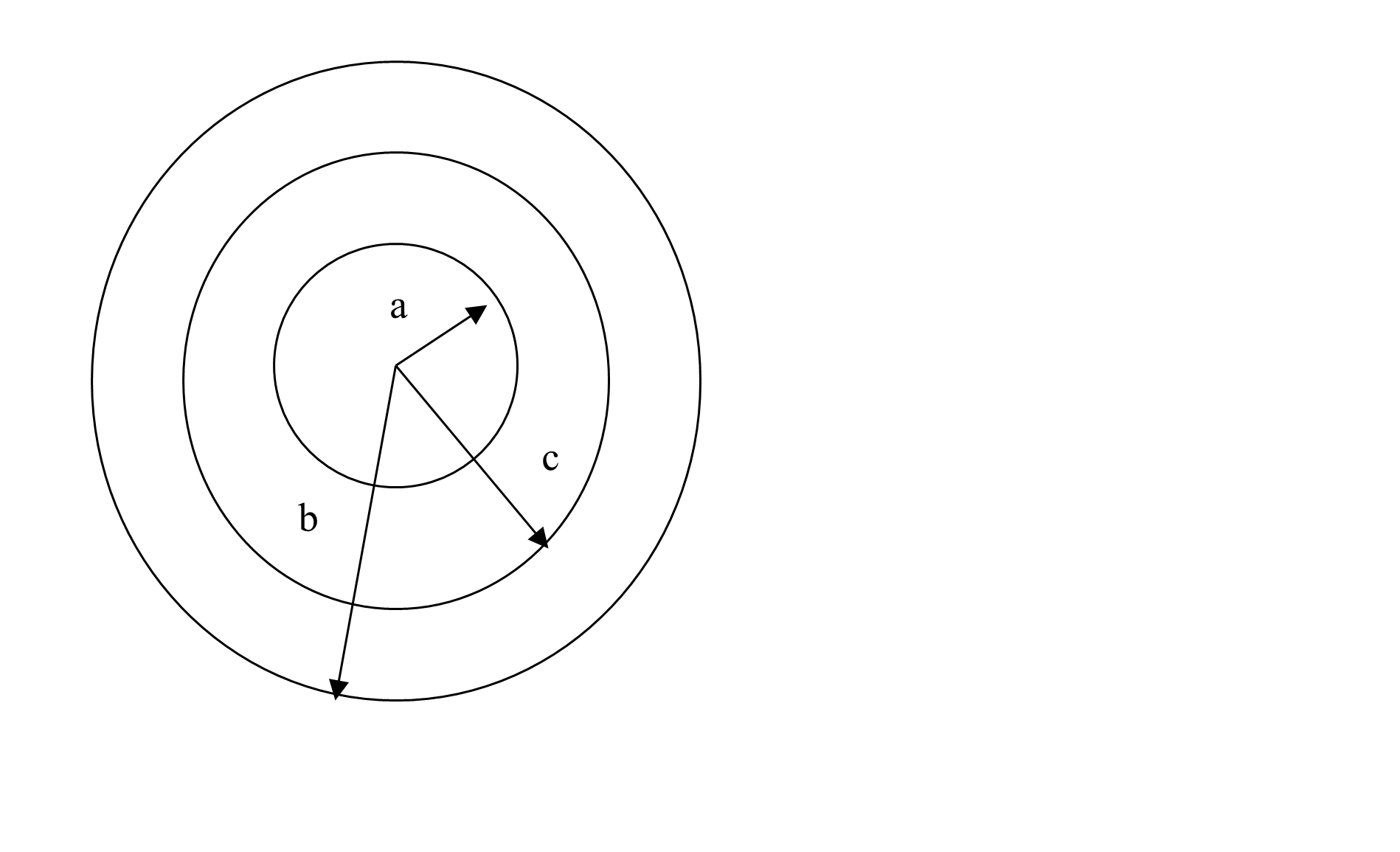
Figure 2 A compounded cylinder pressure vessel with internal radius, \(a\), outer radius, \(b\), and interface at \(r = c\).
Let us make the compounded cylinder of two cylinders (Figure 2). Cylinder 1 has an internal radius of \(a = 5^{\prime\prime}\), and outer radius \(c = 6.5^{\prime\prime}\), while Cylinder 2 has an internal radius of \(c = 6.5^{\prime\prime}\) and outer radius, \(b = 8^{\prime\prime}\). Assume that that radial interference, \(\delta = 0.007^{\prime\prime}\) occurs at the interface of a compounded cylinder at \(r = c = 6.5^{\prime\prime}\). How does then one find the pressure that can be applied to the compounded cylinder of internal radius, \(a = 5^{\prime\prime}\) and outer radius, \(b = 8^{\prime\prime}\)?
For cylinder 1, the radial displacement, \(u_{1}\) is given by
\[u_{1} = c_{1}r + \frac{c_{2}}{r}\;\;\;\;\;\;\;\;\;\;\;\; (4)\]
the radial stress, \(\sigma_{r}^{1}\)and hoop stress, \(\sigma_{\theta}^{1}\) by
\[\sigma_{r}^{1} = \frac{E}{1 - \nu^{2}}\left\lbrack c_{1}\left( 1 + \nu \right) - c_{2}\left( \frac{1 - \nu}{r^{2}} \right) \right\rbrack\;\;\;\;\;\;\;\;\;\;\;\; (5)\]
\[\sigma_{\theta}^{1} = \frac{E}{1 - \nu^{2}}\left\lbrack c_{1}\left( 1 + \nu \right) + c_{2}\left( \frac{1 - \nu}{r^{2}} \right) \right\rbrack\;\;\;\;\;\;\;\;\;\;\;\; (6)\]
where
\[E = \text{Young's modulus of steel,}\]
\[\nu = \text{Poisson's ratio of steel.}\]
For cylinder 2, the radial displacements, \(u_{2}\)is given by
\[u_{2} = c_{3}r + \frac{c_{4}}{r}\;\;\;\;\;\;\;\;\;\;\;\; (7)\]
the radial stress, \(\sigma_{r}^{2}\) and hoop stress, \(\sigma_{\theta}^{2}\) by
\[\sigma_{r}^{2} = \frac{E}{1 - \nu^{2}}\left\lbrack c_{3}\left( 1 + \nu \right) - c_{4}\left( \frac{1 - \nu}{r^{2}} \right) \right\rbrack\;\;\;\;\;\;\;\;\;\;\;\; (8)\]
\[\sigma_{\theta}^{2} = \frac{E}{1 - \nu^{2}}\left\lbrack c_{3}\left( 1 + \nu \right) + c_{4}\left( \frac{1 - \nu}{r^{2}} \right) \right\rbrack\;\;\;\;\;\;\;\;\;\;\;\; (9)\]
So if one is able to find the four constants, \(c_{1},c_{2},c_{3}\) and \(c_{4}\), one can find the stresses in the compounded cylinder to be able to find what internal pressure can be applied. So how do we find the four unknown constants?
The boundary and interface conditions are the following.
The radial stress at the inner radius, \(r = a\) is the applied internal pressure
\[\sigma_{r}^{1}\left( r = a \right) = - p_{i}\;\;\;\;\;\;\;\;\;\;\;\; (10)\]
The radial stress is continuous at the interface, \(r = c\)
\[\sigma_{r}^{1}\left( r = c \right) = \sigma_{r}^{2}\left( r = c \right)\;\;\;\;\;\;\;\;\;\;\;\; (11)\]
The radial displacement at the interface, \(r = c\) has a jump of the radial interference, \(\delta\)
\[u_{2}\left( r = c \right) - u_{1}\left( r = c \right) = \delta\;\;\;\;\;\;\;\;\;\;\;\; (12)\]
The radial stress at the outer radius, \(r = c\) is
\[\sigma_{r}^{2}\left( r = b \right) = 0\;\;\;\;\;\;\;\;\;\;\;\; (13)\]
This will set up four equations and four unknowns, if we know what internal pressure we are applying. Assume we are applying the same pressure as the single cylinder can take, that is,\(p_{i} = 7.887\)ksi and let us see later what stresses it creates in the compounded cylinder.
Assuming \(E = 30 \times 10^{6}\)psi, \(\nu = 0.3\), Equations (10) through (13) become
\[\frac{30 \times 10^{6}}{1 - 0.3^{2}}\left\lbrack c_{1}\left( 1 + 0.3 \right) - c_{2}\left( \frac{1 - 0.3}{5^{2}} \right) \right\rbrack = - 7.887 \times 10^{3}\]
\[\frac{30 \times 10^{6}}{1 - 0.3^{2}}\left\lbrack c_{1}\left( 1 + 0.3 \right) - c_{2}\left( \frac{1 - 0.3}{6.5^{2}} \right) \right\rbrack = \frac{30 \times 10^{6}}{1 - 0.3^{2}}\left\lbrack c_{3}\left( 1 + 0.3 \right) - c_{4}\left( \frac{1 - 0.3}{6.5^{2}} \right) \right\rbrack\]
\[c_{3}\left( 6.5 \right) + \frac{c_{4}}{6.5} - c_{1}\left( 6.5 \right) - \frac{c_{2}}{6.5} = 0.007\]
\[\frac{30 \times 10^{6}}{1 - 0.3^{2}}\left\lbrack c_{3}\left( 1 + 0.3 \right) - c_{4}\left( \frac{1 - 0.3}{8^{2}} \right) \right\rbrack = 0\;\;\;\;\;\;\;\;\;\;\;\; (14a-d)\]
Writing the Equations (14a-d) in matrix form, we get
\[\begin{bmatrix} 4.2857 \times 10^{7} & - 9.2307 \times 10^{5} & 0 & 0 \\ 4.2857 \times 10^{7} & - 5.4619 \times 10^{5} & - 4.2857 \times 10^{7} & 5.4619 \times 10^{5} \\ - 6.5 & - 0.15384 & 6.5 & 0.15384 \\ 0 & 0 & 4.2857 \times 10^{7} & - 3.6057 \times 10^{5} \\ \end{bmatrix}\begin{bmatrix} c_{1} \\ c_{2} \\ c_{3} \\ c_{4} \\ \end{bmatrix} = \begin{bmatrix} - 7.887 \times 10^{3} \\ 0 \\ 0.007 \\ 0 \\ \end{bmatrix}\;\;\;\;\;\;\;\;\;\;\;\; (15)\]
Solving these four simultaneous linear equations, we can find the four constants.
References
(1) A.C. Ugural, S.K. Fenster, Advanced strength and applied elasticity, Third Edition, Prentice Hall, New York, 1995.
(2) J.E. Shigley, C.R. Mischke, Chapter 19 - Limits and fits, Standard handbook of machine design, McGraw-Hill, New York, 1986.
Questions
(1) Find the unknown constants of Equation (14) using different numerical methods.
(2) Knowing that the critical points in the compounded cylinder are \(r = a,c - ,c + ,\text{and}\ b\), find the maximum hoop stress in the compounded cylinder. What is its value compared to the maximum hoop stress allowable of 18 ksi?
(3) Find the maximum internal pressure you can apply to the compounded cylinder? Compare it with the maximum possible internal pressure for a single cylinder of the same dimensions.
(4) The radial interference at the interface is created by making the inner cylinder 1 to have a larger outer radius than the inner radius of cylinder 2. Standard interference fits dictate the limits of these dimensions. If cylinder 2 is fit into cylinder 1, there is an upper and lower limit by which the nominal diameter of each cylinder varies at the interface. This limit L in thousands of an inch, is given by [2]
\[L = CD^{1/3}\] where \(D\) (nominal diameter) is in inches, and the coefficient \(C\),based on the type of fit, is given in Table 1 below.
| Cylinder | Limit | Class of fit | |
|---|---|---|---|
| FN2 | FN3 | ||
| \(1\) | \(\text{Lower}\) | \(0.000\) | \(0.000\) |
| \(\text{Upper}\) | \(0.907\) | \(0.907\) | |
| \(2\) | \(\text{Lower}\) | \(2.717\) | \(3.739\) |
| \(\text{Upper}\) | \(3.288\) | \(4.310\) |
Assuming FN2 fit at the interface, find the maximum internal pressure you would recommend.
Summary
To find the diametrical contraction during shrink-fitting in a trunnion requires one to first find how the coefficient of linear thermal expansion of steel is related to temperature. The relation is given through a second-order polynomial, and calculating the coefficients of the polynomial requires solving a set of simultaneous linear equations.
Modeling
To make the fulcrum (Figure 1) of a bascule bridge, a long hollow steel shaft called the trunnion is shrink fit into a steel hub. The resulting steel trunnion-hub assembly is then shrunk-fit into the girder of the bridge.
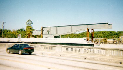
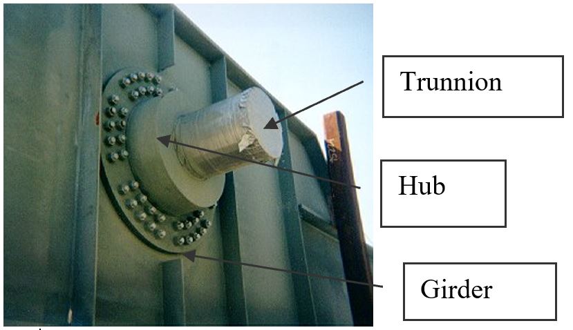
Figure 1 Trunnion-Hub-Girder (THG) assembly.
This is done by first immersing the trunnion in a cold medium such as dry-ice/alcohol mixture. After the trunnion reaches the steady-state temperature, that is, the temperature of the cold medium, the trunnion outer diameter contracts. The trunnion is taken out of the medium and slid through the hole of the hub (Figure 2).
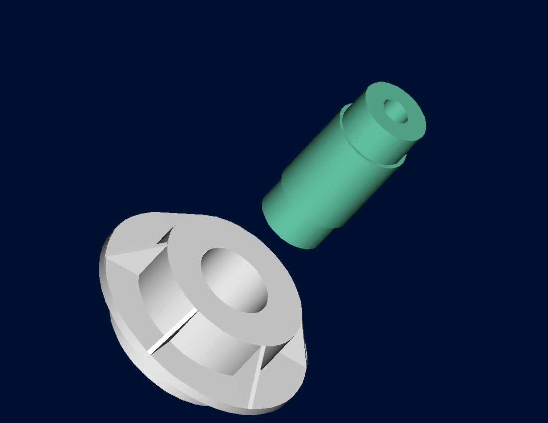
Figure 2 Trunnion slid through the hub after contracting
When the trunnion heats up, it expands and creates an interference fit with the hub. In 1995, on one of the bridges in Florida, this assembly procedure did not work as designed. Before the trunnion could be inserted fully into the hub, the trunnion got stuck. Luckily the trunnion was taken out before it got stuck permanently. Otherwise, a new trunnion and hub would be needed to be ordered at a cost of $50,000. Coupled with construction delays, the total loss could have been more than a hundred thousand dollars.
Why did the trunnion get stuck? This was because the trunnion had not contracted enough to slide through the hole. Can you find out why?
A hollow trunnion of an outside diameter \(12.363^{\prime\prime}\) is to be fitted in a hub of an inner diameter \(12.358^{\prime\prime}\). The trunnion was put in dry-ice/alcohol mixture (temperature of the fluid - dry ice/alcohol mixture is \(- 108{^\circ}\text{F}\)) to contract the trunnion so that it can be slided through the hole of the hub. To slide the trunnion without sticking, a diametrical clearance of at least \(0.01^{\prime\prime}\) is required between the trunnion and the hub. Assuming the room temperature is \(80{^\circ}\text{F}\), is immersing it in dry-ice/alcohol mixture a correct decision?
Solution
To calculate the contraction in the diameter of the trunnion, the coefficient of linear thermal expansion at room temperature is used. In that case, the reduction, \({\Delta D}\) in the outer diameter of the trunnion is
\[\Delta D = D\alpha\Delta T\ \ \ (1)\]
where
\[D = \text{outer diameter of the trunnion,}\]
\[\alpha = \text{coefficient of linear thermal expansion at room temperature, and}\]
\[\Delta T = \text{change in temperature,}\]
Given
\[D = 12.363^{\prime\prime}\]
\[\alpha = 6.817 \times 10^{- 6}{in/in/}{^\circ}\text{F}\ \text{at}\ 80{^\circ}\text{F}\]
\[\begin{split} \Delta T&= T_{{fluid}} - T_{{room}}\\ &= - 108 - 80\\ &= - 188{^\circ}\text{F} \end{split}\] where
\[T_{{fluid}}= \text{temperature of dry-ice/alcohol mixture}\]
\[T_{{room}}= \text{room temperature}\]
the reduction in the trunnion outer diameter is given by
\[\begin{split} \Delta D &= (12.363)\left( 6.47 \times 10^{- 6} \right)\left( - 188 \right)\\ &=- 0.01504^{\prime\prime} \end{split}\]
So, the trunnion is predicted to reduce in diameter by \(0.01504^{\prime\prime}\). But is this enough reduction in diameter? As per specifications, he needs the trunnion to contract by
\[\begin{split} &= \text{trunnion outside diameter} - \text{hub inner diameter} + \text{diametral clearance} \\ &= 12.363^{\prime\prime} - 12.358^{\prime\prime} + 0.01^{\prime\prime}\\ &= 0.015^{\prime\prime} \end{split}\]
So, according to his calculations, immersing the steel trunnion in dry-ice/alcohol mixture gives the desired contraction of \(0.015^{\prime\prime}\) as we predict a contraction of \(0.01504^{\prime\prime}\).
But as shown in Figure 3, the coefficient of linear thermal expansion of steel decreases with temperature and is not constant over the range of temperature the trunnion goes through. Hence, Equation 1 would overestimate the thermal contraction.
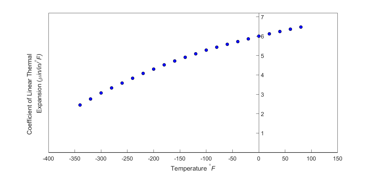
Figure 3 Varying coefficient of linear thermal expansion as a function of temperature for cast steel.
The contraction in the diameter for the trunnion for which the coefficient of linear thermal expansion varies as a function of temperature is given by
\[\Delta D = D\int_{T_{{room}}}^{T_{{fluid}}}{\alpha dT}\ \ \ (2)\]
So one needs to find the curve to find the coefficient of linear thermal expansion as a function of temperature. This curve is found by regression, where we best fit a polynomial through the data given in Table 1.
Table 1 Coefficient of linear thermal expansion as a function of temperature.
| Temperature | Coefficient of linear thermal expansion |
|---|---|
| \({^\circ}\text{F}\) | \({\mu }\text{in/in}/{^\circ}\text{F}\) |
| \(80\) | \(6.47\) |
| \(60\) | \(6.36\) |
| \(40\) | \(6.24\) |
| \(20\) | \(6.12\) |
| \(0\) | \(6.00\) |
| \(-20\) | \(5.86\) |
| \(-40\) | \(5.72\) |
| \(-60\) | \(5.58\) |
| \(-100\) | \(5.28\) |
| \(-120\) | \(5.09\) |
| \(-140\) | \(4.91\) |
| \(-160\) | \(4.72\) |
| \(-180\) | \(4.52\) |
| \(-200\) | \(4.30\) |
| \(-220\) | \(4.08\) |
| \(-240\) | \(3.83\) |
| \(-260\) | \(3.58\) |
| \(-280\) | \(3.33\) |
| \(-300\) | \(3.07\) |
| \(-320\) | \(2.76\) |
| \(-340\) | \(2.45\) |
Assuming that the coefficient of linear thermal expansion is related to temperature by a second-order polynomial,
\[\alpha = a_{0} + a_{1}T + a_{2}T^{2}\ \ \ (3)\]
Given the data points \(\left( \alpha_{1},T_{1} \right)\), \(\left( \alpha_{2},T_{2} \right)\), …..,\(\left( \alpha_{n},T_{n} \right)\) as in Figure 3 and Table 1, the sum of the square of the residuals (sum of the square of the differences between the observed and predicted values) is \[\begin{split} S_{r} &= \sum_{i = 1}^{n}\left( \alpha_{i} - \{ a_{0} + a_{1}T_{i} + a_{2}T_{i}^{2}\} \right)^{2}\\ &= \sum_{i = 1}^{n}\left( \alpha_{i} - a_{0} - a_{1}T_{i} - a_{2}T_{i}^{2} \right)^{2} \ \ \ (4) \end{split}\]
To minimize the value of the sum of the square of the residuals, we take the derivative with respect to each of the three unknown coefficients, \(a_0,\) \(a_1,\) and \(a_2\) to give
\[\begin{split} \frac{\partial S_{r}}{\partial a_{0}} &= \sum_{i = 1}^{n}{2\left( \alpha_{i} - a_{0} - a_{1}T_{i} - a_{2}T_{i}^{2} \right)}\left( - 1 \right)\\ &= 2\left\lbrack - \sum_{i = 1}^{n}\alpha_{i} + na_{0} + a_{1}\sum_{i = 1}^{n}T_{i} + a_{2}\sum_{i = 1}^{n}T_{i}^{2} \right\rbrack \end{split}\]
\[\begin{split} \frac{\partial S_{r}}{\partial a_{1}} &= \sum_{i = 1}^{n}{2\left( \alpha_{i} - a_{0} - a_{1}T_{i} - a_{2}T_{i}^{2} \right)}\left( - T_{i} \right)\\ &= 2\left\lbrack - \sum_{i = 1}^{n}{\alpha_{i}T_{i}} + a_{0}\sum_{i = 1}^{n}T_{i} + a_{1}\sum_{i = 1}^{n}{T_{i}}^{2} + a_{2}\sum_{i = 1}^{n}T_{i}^{3} \right\rbrack \end{split}\]
\[\begin{split} \frac{\partial S_{r}}{\partial a_{2}} &= \sum_{i = 1}^{n}{2\left( \alpha_{i} - a_{0} - a_{1}T_{i} - a_{2}T_{i}^{2} \right)}\left( - T_{i}^{2} \right)\\ &= 2\left\lbrack - \sum_{i = 1}^{n}{\alpha_{i}{T_{i}}^{2}} + a_{0}\sum_{i = 1}^{n}{T_{i}}^{2} + a_{1}\sum_{i = 1}^{n}T_{i}^{3} + a_{2}\sum_{i = 1}^{n}T_{i}^{4} \right\rbrack\ \ \ (5) \end{split}\]
Setting three partial derivatives in Equation (5) equal to zero gives,
\[na_{0} + a_{1}\sum_{i = 1}^{n}{T_{i} + a_{2}\sum_{i = 1}^{n}T_{i}^{2} = \sum_{i = 1}^{n}\alpha_{i}}\]
\[a_{0}\sum_{i = 1}^{n}T_{i} + a_{1}\sum_{i = 1}^{n}T_{i}^{2} + a_{2}\sum_{i = 1}^{n}T_{i}^{3} = \sum_{i = 1}^{n}{\alpha_{i}T_{i}}\]
\[a_{0}\sum_{i = 1}^{n}T_{i}^{2} + a_{1}\sum_{i = 1}^{n}T_{i}^{3} + a_{2}\sum_{i = 1}^{n}T_{i}^{4} = \sum_{i = 1}^{n}{\alpha_{i}T_{i}^{2}}\ \ \ (6)\]
The set of equations given by equations(6a), (6b), and (6c) are simultaneous linear equations. The number of data points in Figure (3) is \(24,\) as given in Table 1. Hence
\[n = 24\]
\[\sum_{i = 1}^{24}T_{i} = - 2860\]
\[\sum_{i = 1}^{24}T_{i}^{2} = 7.26 \times 10^{5}\]
\[\sum_{i = 1}^{24}T_{i}^{3} = - 1.86472 \times 10^{8}\]
\[\sum_{i = 1}^{24}T_{i}^{4} = 5.24357 \times 10^{10}\]
\[\sum_{i = 1}^{24}\alpha_{i} = 1.057 \times 10^{- 4}\]
\[\sum_{i = 1}^{24}\alpha_{i}T_{i} = - 1.04162 \times 10^{- 2}\]
\[\sum_{i = 1}^{24}\alpha_{i}T_{i}^{2} = 2.56799\]
\[\begin{split} &24a_{0} - 2860a_{1} + 7.26 \times 10^{5}a_{2} = 1.057 \times 10^{- 4}\\ &- 2860a_{0} + 7.26 \times 10^{5}a_{1} - 1.8647 \times 10^{8}a_{2} = - 1.04162 \times 10^{- 2}\\ &7.26 \times 10^{5}a_{0} - 1.86472 \times 10^{8}a_{1} + 5.24357 \times 10^{10}a_{2} = 2.56799 \end{split}\;\;\;\;\;\;\;\;\;\;\;\; (7)\]
In matrix form, the three simultaneous linear equations can be written as
\[\begin{bmatrix} 24 & - 2860 & 7.26 \times 10^{5} \\ - 2860 & 7.26 \times 10^{5} & - 1.86472 \times 10^{8} \\ 7.26 \times 10^{5} & - 1.86472 \times 10^{8} & 5.24357 \times 10^{10} \\ \end{bmatrix}\begin{bmatrix} a_{0} \\ a_{1} \\ a_{2} \\ \end{bmatrix} = \begin{bmatrix} 1.057 \times 10^{- 4} \\ - 1.04162 \times 10^{- 2} \\ 2.56799 \\ \end{bmatrix}\;\;\;\;\;\;\;\;\;\;\;\; (8)\]
Questions
(1) Can you now find the contraction in the trunnion outer diameter?
(2) Is the magnitude of contraction more than \(0.015^{\prime\prime}\) as required?
(3) If that is not the case, what if the trunnion were immersed in liquid nitrogen (boiling temperature=\(- 321{^\circ}\text{F}\))? Will that give enough contraction in the trunnion?
(4) Redo problem #1 using a third-order polynomial as the regression model. How much different is the estimate of contraction using the third-order polynomial?
(5) Find the optimum polynomial order to use for the regression model.
(6) Find the effect of the number of significant digits used in solving the set of the equations for problem #4 as you must have noticed that the order of the numbers in the coefficient matrix varies quite a bit.